Solvers¶

Underneath every layer is the same stack: a linear operator that knows how to apply itself but need not store itself, a Newton iteration built on it, and a selection rule that picks a linear backend on measured evidence.

The `LinearOperator` contract¶

Operators are matvec-free. An operator must apply itself; everything else is optional and advertised:

class LinearOperator(Protocol):
    shape: tuple[int, ...]
    dtype: torch.dtype
    device: torch.device
    symmetric: bool

    def matvec(self, x: Tensor) -> Tensor: ...
    def rmatvec(self, x: Tensor) -> Tensor: ...
    def diagonal(self) -> Tensor: ...              # for Jacobi preconditioning
    def assemble(self) -> Tensor | None: ...       # dense form, if it has one
    def spd_certificate(self) -> Tensor | None: ...

An operator may additionally implement assemble_sparse() -> (row, col, values) — the SparseAssembling protocol — which is what unlocks the sparse-direct backend.

Three implementations ship:

Operator	What it represents
`DenseOperator`	A plain matrix. The retained reference against which the others are checked.
`GraphLaplacianOperator`	\(A_I \operatorname{diag}(g) A_I^\top\), built from `endpoints` and `accumulate` — never forming \(A\). This is the Jacobian of a Kirchhoff layer.
`AdvectionOperator`	The upwind advection operator a transport layer solves against.

The point of the contract is that a network with \(10^5\) edges assembles an \(O(E)\) sparse triplet or applies itself in \(O(E)\) work, and never materialises an \(n \times b\) dense matrix.

The SPD certificate¶

spd_certificate() returns a tensor, or None for "cannot say". This drives backend selection, and it is deliberately conservative: an operator asserts SPD only when it can prove it.

GraphLaplacianOperator certifies when its conductances are positive and the interior is grounded. _DiagonalShifted — the Jacobian of a layer carrying potential-dependent nodal sources — delegates to the Laplacian and keeps the certificate only when every shift entry is non-negative: a non-negative diagonal added to an SPD matrix is SPD, a negative one might not be, so the certificate is dropped rather than asserted. The solve then routes to GMRES, which needs none.

Grounding¶

noodl.solvers.grounding provides spd_certificate and spd_diagnosis. The second is the useful one when something goes wrong: a potential problem needs one grounded (boundary) node per connected component, and a network that has lost grounding — a fan reaching shutoff, a damper closing, a component that turns out to be isolated — produces a singular operator. spd_diagnosis names which component is ungrounded rather than leaving you with a failed solve.

This can happen mid-iteration, which is why newton takes a where label and every layer passes something specific like "KirchhoffLayer 'air' solve". In a composed model over one network, a bare "newton: did not converge" is not enough to find the culprit.

`solve`: the `auto` table¶

from noodl.solvers.select import solve

result = solve(op, b, method="auto", rtol=1e-10, on_failure="raise")

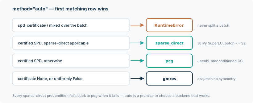
The auto eligibility table resolving to sparse_direct, pcg or gmres

method="auto" resolves by this table, top to bottom, first match wins:

Condition	Backend
`spd_certificate()` mixed across the batch	`RuntimeError` — never split a batch
Certified SPD, and sparse-direct applicable	`sparse_direct` (SciPy SuperLU, per instance)
Certified SPD, otherwise	`pcg` (Jacobi-preconditioned conjugate gradients)
Certificate `None`, or uniformly `False`	`gmres` (assumes no symmetry)

"Sparse-direct applicable" is a conjunction: the operator declares assemble_sparse and returns a sparse form from it, SciPy is importable, the solve is grad-safe, and the flat batch size is at most 32. Every one of those is a fall back to PCG when it fails, never a refusal — auto is a promise to choose a backend that works.

Why that default, and why the batch threshold¶

Measured on the reference composed model (1028 unknowns, ~5300 nonzeros, float64, 14 threads, median of 3 warm runs):

Pass	Ensemble	PCG	sparse-direct
forward	1	128.4 ms	28.0 ms	4.59x faster
forward	100	2399 ms	2182 ms	a tie
forward	1000	29489 ms	19263 ms	1.53x faster
backward	1	44.9 ms	13.8 ms	3.25x faster
backward	100	1741 ms	476 ms	3.66x faster

PCG needed 168–180 iterations per Newton step at this conditioning; the factorisation needs one. But SuperLU is driven by a per-instance Python loop whose cost is linear in the ensemble, while PCG's batched arithmetic is sub-linear — hence the threshold at 32 rather than an unconditional preference. A batched vendor backend would replace the loop, not the algorithm.

Because the choice depends on runtime predicates a caller cannot otherwise observe — the batch size, and whether SciPy is importable at all — diagnostics reports method (what you asked for) and backend (what ran) separately. Without that distinction, an installation missing the sparse extra looks identical to one that has it, at 4.6x the cost.

Failure¶

pcg and gmres never raise. select.solve is the single layer where a failed numerical solve becomes an exception, and on_failure="return" is the narrow escape hatch that returns a SolveResult instead.

An eligibility refusal is different and always raises, whatever on_failure says: requesting method="cg" on an operator that cannot certify SPD, or letting auto see a batch where some but not all instances certify, is a modelling error, not a numerical one. There is no per-instance result to return.

SolveResult carries x, converged, iterations, residual and status per instance, with status one of CONVERGED, MAX_ITER, BREAKDOWN, SINGULAR. raise_on_failure(where) names every non-converged batch index with its status and residual, and returns self when all converged, so it chains.

Newton¶

from noodl.solvers.newton import newton

result = newton(residual, operator, x0, atol=None, rtol=None, max_iter=50,
                omega=0.75, switch_ratio=0.5, method="auto", where="my solve")

Damped, batched Newton. NewtonResult carries x, converged (per instance), iterations, residual_norm, linear_iterations and backend.

Tolerance defaults. atol and rtol both default to None, meaning derive from the working dtype: each independently becomes \(\sqrt{\varepsilon}\) for the dtype of the residual tensor actually returned — about 1.2e-4 for float32, 1.5e-8 for float64. This is the standard "half the significant digits" heuristic. Asking for tighter than that requests precision the dtype does not have: the residual floors below the target and converged never becomes true. An explicit value always overrides, and the two are independent.

linear_iterations is, per instance, the maximum inner-solver count over the Newton steps taken — the worst single linear solve. That is what a performance budget or a preconditioner decision is made against, and it is monotone in problem difficulty in a way a sum over a varying number of steps is not. It is None only when no linear solve happened at all, never as a stand-in for an unknown count.

Convergence is per batch instance, and the mask is computed on detached copies so it never enters the autograd graph.

Kinked monotone laws: line_search="convex". When every branch flow is non-decreasing in its own potential difference and every nodal withdrawal in its own potential, the residual is the gradient of a convex function \(E\) and the Newton direction is a descent direction of \(E\). A law with kinks (a flat-steep-flat S-curve, a stiff bed meeting a soft storage line) can still send the damped Newton into a cycle it never leaves, because the step crosses a kink and lands past the minimum of \(E\) along it. With line_search="convex" such a step, recognised by the directional derivative \(\phi'(t) = r(x + t d)\cdot d\) at its end, is cut back to that minimum by a regula falsi on the monotone \(\phi'\); a step that does not overshoot is taken unchanged, so a smooth solve is bitwise the same.

Round-off floor: step_floor. An atol below the round-off of the residual's own terms (a stiff law at a large potential) cannot be met: the iterate stands still and the solve fails. step_floor=k ends an instance as converged once its Newton step is within k ULPs of the iterate in every component, i.e. at the floor. Both options are off by default; a layer that needs them sets them as its newton_defaults (the sewer's dynamic wave does).

Monotone scalar solves¶

noodl.solvers.scalar.solve_monotone is a batched bracketed root-finder for a scalar equation known to be monotone. It appears wherever a closed-form inversion does not exist but monotonicity is provable:

The sewer's Manning normal-depth inversion — discharge is strictly increasing in depth up to \(h/D = 0.938\), so the ascending branch is the entire invertible domain.
The sewer's implicit-Euler storage sweep.
The water application's Hazen-Williams inversion with a minor-loss term.
AllocatedFlowLayer's projection-mode QP, whose KKT stationarity reduces to one scalar monotone equation per node.

Monotonicity is what makes bracketing safe, and each caller documents why it holds.

Implicit solve and the adjoint¶

noodl.solvers.implicit is what makes the whole package differentiable at reasonable cost. implicit_solve wraps a Newton solve in a torch.autograd.Function whose backward applies the implicit-function theorem at the converged solution rather than unrolling the forward iteration. adjoint solves the transposed system, using TransposeOperator to present any operator's rmatvec as a forward action.

The cost is one extra linear solve on the backward pass, independent of how many Newton iterations the forward took. Differentiability covers what this means for your model.