Sewers

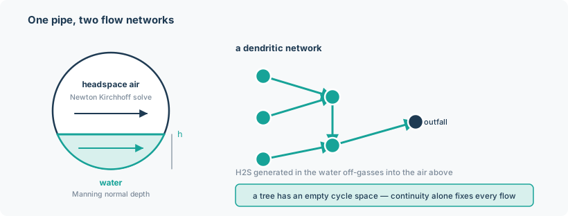
Gravity sewer networks, with the water, the air above it and the sulfide it carries coupled on one network. Manholes are nodes and circular pipes are edges, draining as a tree to an outfall; wastewater flows downhill under gravity, and the question the model answers is corrosion and odour risk: how much H₂S is generated, and how much reaches the air where it attacks the crown of the pipe.

Three physical subsystems share the network, each conserving its own quantity at every manhole — water volume, headspace air, and BOD and sulfide mass — and each uses a different part of the framework:

• Water hydraulics — partially full circular pipes under gravity. Under kinematic-wave routing, Manning's equation on a dendritic network: the cycle space is empty, so continuity alone fixes every discharge in closed form, with no potential solve at all. Under dynamic-wave routing, SWMM's momentum equation as a Kirchhoff layer on head (see Dynamic wave), which admits backwater, flat conduits and loops.
• Headspace air — the air above the water surface is its own flow network, a full KirchhoffLayer driven by wall friction, the drag of the moving water surface, and buoyancy from the sewer-to-ambient temperature difference, vented through manhole leaks and optional fans.
• Water quality — BOD decay and Pomeroy–Parkhurst sulfide generation in the wastewater, with two-film Henry's-law transfer of H₂S into the headspace air, as two coupled transport layers.

Units. Water and headspace air flow m³/s, depth and head m, pressure Pa, concentrations kg/m³ (with helpers to mg/L and ppm), sulfide transfer kg S/s.

from noodl.apps.sewer import (
    SewerNetwork, Manhole, Pipe, Outfall, tree_steady,
    build_model, sewer_steady, initial_state,
    pipe_table, to_ppm, to_mg_per_litre,
)

Every type this application offers — what it does and how to call it — is listed in its catalogue. It is set up and run like every other model; see Using noodl.

A worked example

from noodl.apps.sewer import build_model, sewer_steady, pipe_table, tree_steady

model, state, drivers = build_model(tree_steady())
final = sewer_steady(model, state, drivers)
rows = pipe_table(model, final, drivers, path="pipes.csv")

# rows[0] is pipe "C1": q = 0.05 m3/s, h = 0.153007001 m

(From tests/apps/sewer/test_report.py.) tree_steady() is the committed 5-conduit, 6-node fixture; its steady discharges are 0.05, 0.08, 0.03, 0.13 and 0.16 m³/s.

Start from a different state by naming it — here, sulfide already present in manhole J1 — and read the result by manhole and species:

from noodl.apps.sewer import initial_state

wq = model.refs.water_quality                  # species ("bod", "sulfide"), kg/m3
start = initial_state(model, drivers=drivers, values={wq.concentration: {"J1": {"sulfide": 1e-3}}})
model.check(start, drivers).raise_for_errors(strict=True)
after = model.step(start, drivers, 60.0)
print(sorted(wq.concentration.named(after[wq.concentration])))

['J1', 'J2', 'J3', 'J4', 'J5']

The sewer's initial_state takes the drivers as well (drivers=), because the storage it starts from depends on the inflows. In the dictionaries the concentrations are "water_quality.x" and "air_quality.x" (manhole order, species last); see Using noodl.

A model can also be read from a SWMM .inp file (see File formats):

from noodl.apps.sewer import read_swmm_inp, build_model

net, inflows, pollutants = read_swmm_inp("tree_steady.inp")
model, state, drivers = build_model(net)

The file's FLOW_UNITS (CFS, GPM, MGD, CMS, LPS or MLD) are converted to noodl's SI as it is read; see the Units paragraph of File formats. A network with no links (no conduits, orifices, weirs or outlets) is refused by build_model by name.

For a single step rather than a steady state:

new = model.step(state, drivers, 60.0)
residuals = model.residuals(new, drivers)     # per-layer nodal balance

Building a network

Object	Fields
Manhole(name, invert, ground=None, inflow=0.0, surface_area=None, surcharge_depth=0.0, initial_depth=0.0, storage=None)	A junction. surface_area defaults to SWMM's MIN_SURFAREA, 1.167 m² — a 4 ft shaft. surcharge_depth, initial_depth and storage are dynamic-wave physics (see "Dynamic wave").
storage_unit(name, invert, max_depth, curve, *, surcharge_depth=0.0, initial_depth=0.0, inflow=0.0)	A SWMM storage unit: a Manhole whose storage is the surface-area curve (("functional", a, b, c) for A = a y^b + c, ("tabular", depths, areas), or ("cylindrical", L, W), ("conical", L, W, Z), ("paraboloid", L, W, H), ("pyramidal", L, W, Z); m and m²) and whose ground is invert + max_depth. Dynamic wave only.
Pipe(name, u, v, length, diameter, n, slope, inlet_offset=0.0, outlet_offset=0.0)	A circular gravity conduit; offsets (m) are the invert heights above the end nodes' inverts.
Outfall(name, invert, kind="free", stage=None, flap_gate=False, tide=None, series=None, stage_series=None)	The root of a tree. kind is "free", "normal", "fixed" (stage, m, required), "tidal" (tide, a SWMM TIDAL curve as (hour, stage m) pairs, required) or "timeseries" (its stage comes from stage_series, the file's series as an inflows.TimeSeries in s and m, held at both ends, or else from the outfall_stage driver; series is the SWMM series' name); only dynamic-wave routing reads them.
Orifice(name, u, v, orientation, shape, height, crest_height, discharge_coefficient, width=None, flap_gate=False)	A SWMM orifice from u to v: orientation "side" or "bottom", shape "circular" (height its diameter, m) or "rectangular" (height, width, m), its crest crest_height m above u's invert, Cd (-). Dynamic wave only.
Weir(name, u, v, kind, height, width, crest_height, discharge_coefficient, side_slopes=(0, 0), end_contractions=0, end_discharge_coefficient=0, can_surcharge=True, flap_gate=False)	A SWMM weir: kind "transverse", "sideflow" (opening width m long), "v_notch" (width the top width) or "trapezoidal" (width the bottom width, side_slopes horizontal per vertical); Cd in SWMM's SI units (m^0.5/s). Dynamic wave only.
Outlet(name, u, v, crest_height, rating, head_difference=False, flap_gate=False)	A SWMM outlet: rating ("functional", a, b) for q = a h^b or ("tabular", heads, flows) (m, m³/s); h the depth above the crest, or the head across it with head_difference. Dynamic wave only.
SewerNetwork(manholes, pipes, outfalls, routing="kinematic_wave", notes={}, dynamic_wave=DynamicWaveOptions(), orifices=(), weirs=(), outlets=())	The whole network. routing is "steady", "kinematic_wave" or "dynamic_wave"; SWMM's STEADY/KINWAVE/DYNWAVE are accepted and normalised.

validate() refuses, by name: duplicate node or pipe names; a pipe naming an unknown node; non-positive slope, diameter, length or roughness; a manhole with anything other than exactly one outgoing pipe; an outfall with an outgoing pipe; and a manhole whose component never reaches an outfall — which also catches cycles. With routing="dynamic_wave" these tree rules are replaced: loops and flat pipes are allowed, the network needs at least one outfall (SWMM's ERR_NO_OUTLETS, flowrout.c:325; nothing is asked of each component, so a junction no link reaches, or a group of nodes without an outfall, is read and routed by its own continuity, filling from its inflow and flooding at its full depth), and each outfall ends exactly one link (a conduit or a regulator). Orifices, weirs and outlets are refused by name for the other routings, and malformed ones (an unknown node, a duplicate link name, a bad shape, a negative crest or coefficient, an unsorted rating) for every routing.

That one-outgoing-pipe rule is the dendritic constraint, and it is what makes the closed-form flow solve valid.

build_model

model, state, drivers = build_model(
    net,
    storage=False,          # implicit-Euler manhole storage sweep
    air=True,               # the headspace layer
    quality=True,           # the two quality layers
    species=("bod", "sulfide"),
    f_air=0.02, f_i=7.49e-4, c_s=1.0,
    leak_area=8e-4, leak_cd=0.6, fans=(),
    coupling="pingpong", scheme="implicit", dt_storage=None,
)

species are matched by name, never by position, so their order does not matter: "bod" decays and, when "sulfide" is also present, sulfide is generated from it; any other name is a passive tracer without reactions. "sulfide" without "bod" and repeated names are refused. The air-quality layer and the water-to-air transfer exist only when "sulfide" is among the species (the air-flow layer is built by air=True regardless); a selection without "bod" has no reaction at all. Every species s has a lateral-inflow concentration driver "<s>_in" (kg/m3, default 0), as in the dynamic-wave builder. A single species (species=("bod",) or ("tracer",)) is held with no species axis, "water_quality.x" of shape (manholes,), as TransportLayer holds any one-species layer; BOD decays on it as it does beside other species, in both builders.

air=False gives the water-only model the SWMM parity rows use. fans names manholes carrying a prescribed extraction (m³/s, positive out).

build_model dispatches on net.routing. A "dynamic_wave" network is built by build_dynamic_wave_model, with iterate_tol (m), iterate_flow_tol (m³/s) and iterate_max (passes) controlling the iteration; left out, they follow the file's HEAD_TOLERANCE and MAX_TRIALS (see Iteration and convergence). For it, air, quality and storage default to False; quality=True adds the water-quality layer of species (see Quality on the dynamic wave); air=True builds the headspace air on the solved conduits (see Headspace air on the dynamic wave) and takes f_air, f_i, c_s, leak_area, leak_cd and fans as above; storage=True, a non-default coupling or dt_storage (kinematic-wave options: the dynamic wave always iterates its passes on its routing step) and a geometry="analytic" network (it always routes on SWMM's tabulated circle) are refused, naming the option; iterate_tol, iterate_flow_tol and iterate_max are refused for the other routings. Run it with simulate_dynamic_wave (see Dynamic wave), not sewer_steady. To tune the iteration itself (relaxation, acceleration, memory), call build_dynamic_wave_model(net, ...) from noodl.apps.sewer directly; it takes the same dynamic-wave arguments as build_model.

dt_storage (optional) declares the interval the manhole storage sweep integrates over. When given, a step at any other interval is refused by name. Omit it (the default) to follow the model's own step interval via the StepContext the closure receives.

initial_state(model, drivers=None) builds the all-zero state, dispatching on each layer's quantity. When drivers is given, it also evaluates the initial storage (by querying model.initial_capacities), which a step with a changing capacity requires to be in the step-start state. Drivers are required for initial_state whenever the model has a quality layer, because the hydraulics closure writes those layers' capacity from the flows and the initial storage must be evaluated from the drivers; this holds with or without storage=True.

sewer_steady(model, state, drivers, *, reaction=None, dt=60.0, max_iter=500, tol=1e-12) steps repeatedly until every transport layer stops changing. You need it rather than Model.steady whenever quality is on, because Model.steady never applies reactions.

model._apply_closures(state, drivers) resolves the hydraulics without stepping any layer, which is the quickest way to inspect sewer.q, sewer.h, sewer.v and the rest.

The physics

Exact circular geometry

With the wetted half-angle \(\theta = 2\arccos(1 - 2h/D)\):

\[ A = \frac{D^2(\theta - \sin\theta)}{8},\quad P = \frac{D\theta}{2},\quad R = \frac{A}{P} = \frac{D}{4}\left(1 - \frac{\sin\theta}{\theta}\right),\quad T = D\sin\frac{\theta}{2} \]

These exact relations are the default for networks built in code (SewerNetwork(..., geometry="analytic")).

SWMM's own circular geometry

SWMM 5 does not evaluate the circle. For a CIRCULAR conduit it interpolates 51-point tables (A/Afull, Y/Yfull and the section factor S/Sfull, from xsect.dat) and near the invert switches to closed forms solved by Newton iterations with their own starting guesses and stopping rule (xsect.c). The tables differ from the true circle by up to ~5e-3 in depth, and by far more in velocity near the invert. geometry="tabulated" (module noodl.apps.sewer.xsect_tables) reproduces all of it, operation for operation, and is what read_swmm_inp uses by default, because a network read from a SWMM file is read to reproduce SWMM (read_swmm_inp(path, geometry="analytic") gives the exact circle).

At a kinematic-wave steady state SWMM gives a conduit carrying \(q\) an inlet area \(a_1 = A(S = q/\beta)\) (inverse section-factor lookup) and an outlet area \(a_2\) solving \(\beta\,S(a_2) = q\). It reports depth \(\tfrac12(Y(a_1) + Y(a_2))\), volume \(\tfrac12(a_1 + a_2)L\), and velocity \(q / A(\text{depth})\), which is zero at a depth of 0.01 ft or less. \(a_1 = a_2\) on the tables. Near the invert the two Newton solves differ slightly, and both are carried. SWMM's units are reproduced too: it computes in feet with Manning's 1.486, but converts CMS flows and volumes with 0.02832 m³/ft³ rather than \(0.3048^3\). That is an effective 1.6e-4 on the Manning coefficient and 1.2e-4 on reported volumes. Everything is differentiable: piecewise-linear tables, unrolled Newton loops, and one implicit-function root.

Scope: on the kinematic path geometry="tabulated" covers the steady case only, and is refused by name with storage=True. Dynamic-wave routing always uses the tables and refuses geometry="analytic" by name. The discharge limit is SWMM's Qfull rather than the analytic 0.938 D capacity. The headspace, top width, hydraulic radius and mean depth (air side, sulfide) of a circular conduit remain the exact circle, evaluated at SWMM's depth. SWMM has no headspace to compare them with. Other shapes are dynamic-wave only (below); the kinematic and steady paths refuse them by name.

Numerical care worth noting: the arccos argument is clamped to the exact domain \([-1, 1]\), not an epsilon-shrunk one — that was tried and rejected because it shifts the boundary value by \(O(\sqrt{\varepsilon})\). Every \(0/0\) site is guarded on both branches of its torch.where, so a masked-out branch cannot back-propagate inf * 0 = nan.

Manning and normal depth

\(Q = \frac{1}{n} A R^{2/3} \sqrt{S_0}\), with the SI constant 1.0. \(Q\) is strictly increasing in \(h\) up to \(h/D = 0.938\) and decreases above it, so the ascending branch is the entire invertible domain. normal_depth inverts it with solve_monotone, batched over pipes and instances.

q = 0 returns exactly h = 0 with gradient 0 — a documented modelling choice, since the true \(dh/dq\) diverges there. A discharge above capacity_flow is refused by name: surcharge and backwater are out of scope.

The storage sweep

With storage=True, each manhole's water level is advanced by implicit Euler:

\[ A_s \frac{H^{n+1} - H^{n}}{\Delta t} + Q_{\text{out}}(H^{n+1}) = \sum Q_{\text{up}} + \text{lateral} \]

solved with solve_monotone bracketed on \([0, 0.938D]\), valid because both left-hand terms are strictly increasing in \(H^{n+1}\). The sweep runs level-synchronously from leaves to outfall using topological levels computed once; the only Python loop is over tree levels (depth 3 on the committed fixture), never over individual pipes. Each level is one gather and one scatter.

When storage=True the normal-depth inversion is skipped entirely — the sweep has already solved each manhole's own level, which is its outgoing pipe's entrance depth, bit-for-bit and with no root-find.

Dynamic wave

With routing="dynamic_wave" (SWMM's DYNWAVE) the network is a Kirchhoff layer on head. Where a conduit's flow follows from continuity alone, as on a dendritic kinematic-wave network, nothing else is needed; where backwater, a flat conduit or a loop makes the flow depend on the heads at both ends, the heads are the unknowns and the flows follow from the head differences. The water side then has one KirchhoffLayer named "water" (quantity head in m, flow in m³/s) over the conduits, with the outfalls as its boundary, and a JunctionStorage node source at every junction.

The rest of this section follows the physics in the order it enters the solve: the equations and how they are solved (iteration, Anderson acceleration and the flow tolerance it needs); the three places where SWMM's own iteration has no fixed point and noodl takes a documented tie rule (the crown hold band of EXTRAN, the normal-flow slope switch and the drop-end area switch); the starting state; surcharge, flooding, storage units, orifices, weirs and outlets and the conduit options; the variable step and time-varying inflow, tidal and time-series outfalls; water quality and headspace air; and last the intentional differences from SWMM. What is not supported is listed once, under Limitations.

Equations

SWMM 5.2.4's conduit and junction updates (dwflow.c, dynwave.c) are solved at their fixed point rather than replayed trial by trial. For one barrel of conduit length \(L\) (m) between heads \(h_1\) and \(h_2\) (m), after a step \(\Delta t\) (s):

\[ q = \frac{q_{\text{old}} + \Delta q_3 + \Delta q_4}{1 + \Delta q_1} + \frac{g\,\Delta t\,A_w}{L\,(1 + \Delta q_1)}\,(h_1 - h_2) \]

where \(q_{\text{old}}\) is the flow at the step start (m³/s), \(\Delta q_1\) the friction and \(\Delta q_3\), \(\Delta q_4\) the convective and area-change momentum terms, and \(A_w\) the weighted flow area (m²) that SWMM forms from the end and mid-conduit areas. The coefficients are evaluated at the converged depths and flow. SWMM's two post-conditions are applied afterwards: the normal-flow limit (NORMAL_FLOW_LIMITED, SLOPE/FROUDE/BOTH/NO), and the dry-node clamps, which zero a flow that would draw from a junction with no water. At a junction that is not an outfall, with surface area \(A_s\) (m², the sum of the surface areas of the conduits meeting there, plus a storage unit's own area, floored at MIN_SURFAREA) and depth \(y\) (m):

\[ A_s\,(y - y_{\text{old}}) = \tfrac12\,\Delta t\,(N_{\text{old}} + N) \]

with \(N\) the net inflow (m³/s: lateral inflow plus the conduit flows into the junction). Outfalls are boundary heads: FREE takes the lesser of normal and critical depth in the outfall conduit, NORMAL its normal depth, FIXED the stage with SWMM's stage logic, each from the flow in that conduit. TIDAL and TIMESERIES outfalls use the same stage logic with a stage that varies in time (see "Tidal and time-series outfalls").

What is solved

For frozen coefficients the conduit and junction equations are linear in the heads apart from the min-clamps, so one pass is a single KirchhoffLayer solve. The model then refreshes the coefficients and repeats until the heads change by less than iterate_tol (m) and the flows by less than iterate_flow_tol (m³/s), or iterate_max passes are used (Model(coupling="iterate"), converging on the layer's own interior head; the defaults follow the file, see Iteration and convergence). The result is the head and flow field at which a SWMM trial reproduces its own input.

The passes are Anderson-accelerated by default (noodl.apps.sewer.build_dynamic_wave_model(net, acceleration="anderson", memory=5); Model's iterate_acceleration, see Layers and models). Each pass's flows must then also reproduce the flows it was fed to within iterate_flow_tol (m³/s): the head solve stops on its warm start once every junction balance is within its atol (solve_atol), so near convergence the heads stand still while the flows of a flat or nearly dry conduit still drift. Against plain relaxation judged on the heads alone the mean passes per step fall from 34.8 to 14.1 (tree), 30.2 to 10.4 (backwater line) and 20.8 to 9.7 (loop) over the first 60 steps, and from 42.8 to 11.3 over the loop's first 120, whose worst step drops from 327 passes to 22. The two iterations land on the same fixed point: with a tight head solve (atol=1e-12) they agree to 2e-12 m; at the default solve_atol each lands within the head solve's own resolution, atol dt / (2 A_s) (a few 1e-9 m). The mixing keeps to the fixed points plain relaxation (and SWMM's relaxed trials) can reach: a flat, near-dry conduit's flow can have a second, repelling fixed point, and a mixed step heading for it is replaced by the relaxed step. acceleration=None is plain relaxation. The flows are judged either way, never the heads alone, because on the normal-flow slope switch (below) the heads bound the flows' residual only weakly, and a heads-only test was measured stopping 3e-5 m³/s short of the fixed point.

SWMM's iteration artefacts are not modelled: trial relaxation, the 0.001 cfs flow-reversal rule and link bypassing. Each is a device for reaching the fixed point and none moves it.

Iteration and convergence

HEAD_TOLERANCE and MAX_TRIALS are read into DynamicWaveOptions and are the defaults of the iteration (noodl.apps.sewer.dynwave.iterate_tolerances); an explicit iterate_tol, iterate_flow_tol or iterate_max overrides each:

control	default	SWMM
iterate_tol (m)	HEAD_TOLERANCE (the file's length unit), else 0.005 ft = 0.001524 m	the same test: every node's depth change between trials (dynwave.c::findNodeDepths)
iterate_flow_tol (m³/s)	\(2 A_{\min} \epsilon_H / \Delta t\) (\(\epsilon_H\) = iterate_tol), at least 1e-10	none: SWMM judges the heads alone
iterate_max (passes)	MAX_TRIALS, else 8 (at least 2)	the same limit

The flow tolerance is the flow residual that matches the head tolerance: a flow error \(dQ\) moves a junction's next depth by \(\Delta t\, dQ / (2 A_s)\) (the trapezoid), so at the surface-area floor \(A_{\min}\) (MIN_SURFAREA, 12.566 ft² by default) and the routing step \(\Delta t\) it is a move of exactly iterate_tol, and less at every larger junction. At SWMM's defaults on a 5 s step that is 7.1e-4 m³/s.

A step that uses up the file's trials is accepted, as SWMM accepts it (it counts it as "not converging", NonConvergeCount): the step is taken with its last pass, its diagnostics say converged False, and simulate_dynamic_wave returns out["converged"] per step, so (~out["converged"]).sum() is SWMM's count. With an explicit iterate_max such a step is refused by name, as before, and a step that has to be differentiated is always refused when it does not converge (there is no fixed point to differentiate).

The head solve within a pass. Every law of a pass is non-decreasing in its own head difference (conduits, regulators) or head (junction withdrawals), so the head solve's residual is the gradient of a convex function, and the layer's Newton runs with line_search="convex" and step_floor=16 (dynwave.HEAD_SOLVE_NEWTON; see Solvers). The first cuts back a step that overshoots across a kink: the stiff bed below a dry junction's invert met by a fast inflow, the normal-flow switch's flat-steep-flat flow, the hold band and flood wall. A damped Newton step there could fall into a 2-cycle it never left, and the run stopped with "failed to converge after 50 iterations" (13 files of the SWMM corpus did, among them a junction fed down a 20 m drop and a looped siphon). The second ends a solve whose residual sits at the round-off of its own terms above solve_atol (a junction flooding 17 m above its outfall behind a 0.1 m³/s cap, or a large storage area at a high head), which failed every step before. A pass whose head solve still stops short is one iterate of the pass iteration, not the end of the step: it hands back its last Newton iterate, is never judged converged, and the iteration goes on from it (Model, on_failure="return_primal"); a differentiated solve still raises. tests/verification/test_sewer_dynwave_parity.py runs both kinds against SWMM (robust_orifice_dynwave.inp at every step, robust_drop_dynwave.inp until SWMM's own first non-converging step).

Measured at SWMM's defaults (the fixtures with HEAD_TOLERANCE and MAX_TRIALS removed, 30 min), against SWMM 5.2.4's own 2.02 trials per step on the tree:

network	passes per step	steps at the limit	worst depth against the tight fixed point (m)	SWMM at its defaults, same measure (m)
tree	2.06	1 / 360	1.6e-3	2.3e-3
backwater	2.22	1 / 360	6.9e-3	1.3e-2
loop	2.01	0 / 360	7.0e-4	3.6e-3
structures	2.39	0 / 360	4.4e-4	5.9e-3
storage	2.06	1 / 360	1.0e-3	2.3e-3

So noodl at SWMM's tolerances is at least as close to the converged answer as SWMM is, in about SWMM's number of trials. A judgement on the flows at 1e-4 m³/s instead takes 2.54 passes on the tree for a 7.8e-5 m answer; the parity tests pass their own tight tolerances (1e-13 m, 2000 passes) and the fixtures set HEAD_TOLERANCE 1e-12 and MAX_TRIALS 500.

Speed. One pass costs a nearly fixed few thousand small tensor operations, whatever the network's size: 10-15 ms on the 6-node tree, from 37 ms, and 38 ms on a 2,047-conduit tree, from 55 ms (benchmarks/sewer_dynwave_speed.py, which also times SWMM). With SWMM's own tolerances the tree's 30 minutes take 11.5 s (123 s before), about 850 times SWMM; the 2,047-conduit tree is about 40 times SWMM. Most of it is the conduit update (dynwave_terms.conduit_terms), SWMM's normal and critical depths, and the head solve, whose Newton Jacobian is the elements' own analytic dflow on the primal passes (KirchhoffLayer(analytic_primal=True); the implicit adjoint still differentiates the converged pass). A batch of B scenarios (simulate_dynamic_wave with a (B, n) inflow) costs about the same per pass, so an ensemble amortises it.

Units

SWMM computes in feet with \(g = 32.2\) ft/s² and Manning's 1.486, and the conduit coefficients here are evaluated exactly that way (reusing xsect_tables.LCF, QCF, PHI). Outputs are converted with SWMM's own factors: head in m is ft × LCF, flow in m³/s is cfs × QCF, conveyance in m²/s is ft²/s × QCF/LCF, and an area in m² is ft² × QCF/LCF, which is the area kinwave_steady reports and makes \(A_s\,\Delta y = \tfrac12\Delta t\,N\) exact in m and m³/s.

Bed stiffening and lagged pieces

SWMM clamps a junction depth at 0 after the update. JunctionStorage stands in for that with a stiff bed term, \(K_{\text{bed}} = 10^{6}\) times the storage slope applied to \(\min(H - z_{\text{bed}}, 0)\), built on MIN_SURFAREA rather than on the pass's \(A_s\). The slope of a junction's balance is therefore positive everywhere, so each junction is grounded by itself and the Jacobian stays symmetric positive definite. The default Newton tolerance solve_atol (m³/s) is scaled per model to the round-off floor of that term (about 2.5e-9 m³/s, or about 5e-9 m of head, on the committed fixtures; it grows with invert elevation).

Some quantities are taken from the previous pass, as SWMM takes them from the previous trial, and are consistent at the fixed point: the flow class and the weighting \(f_{\text{asnh}}\), the surface areas \(A_s\), the normal-flow-limit flag (its Froude test uses the momentum flow at the fed heads; its slope test is applied within the pass where it can be, see the next section), the normal flow, the dry-node flags, the outfall heads (the surface areas' jump at a drop end is applied within the pass where it can have no fixed point, see "Drop-end area switch"), and the head at any conduit end SWMM pins (the head is raised to the invert plus offset when it lies below it, and set to critical depth in UP_CRITICAL/DN_CRITICAL). A conduit with a pinned end has no head dependence there: its conveyance is zero and the pinned head enters the constant term.

Normal-flow slope switch

SWMM limits a conduit's flow to the normal flow \(q_{\text{norm}}\) at its upstream depth when its slope test \(y_1 < y_2\) passes (dwflow.c:637-686; always on for a conduit at an outfall, and under NORMAL_FLOW_LIMITED SLOPE or BOTH). With both end depths inside their clamps that test is \(h_1 - h_2 < z_1 - z_2\) (the conduit-end inverts), a switch on the conduit's own head difference, so DynamicWaveConduit applies it within the head solve instead of from the previous pass:

\[ q = \min\!\big(q_{\text{lin}},\ \max(q_{\text{norm}},\ q_{\text{last}} + S\,(h_1 - h_2 - z_1 + z_2))\big) \]

with \(q_{\text{lin}}\) the momentum flow above, \(q_{\text{last}}\) the previous pass's flow and \(S\) (m²/s) a wall slope. At a fixed point (\(q = q_{\text{last}}\)) this is SWMM's unlimited flow above the switch and its limited flow below it, so every SWMM fixed point is unchanged. It has one more kind of fixed point: on the switching surface \(y_1 = y_2\), with the flow between \(q_{\text{norm}}\) and \(q_{\text{lin}}\). That is the tie rule for the case where SWMM has no fixed point, which a draining network reaches at its outfall conduit. A FREE or NORMAL outfall's depth is set from its conduit's flow, and the limited flow is Manning's normal flow at the upstream depth \(y_1\), at which the outfall's normal depth is \(y_1\) again, up to the interpolation mismatch of SWMM's tables (about 1e-5 m). Once the junction upstream has fallen to the outfall's depth, the limited side is consistent only where that mismatch happens to put the outfall above the junction, and the unlimited side's larger flow raises the outfall above it. SWMM's trials then alternate around the surface: on the tree fixture with every inflow ramped down, SWMM 5.2.4 at HEAD_TOLERANCE 1e-12 m and 500 trials fails to converge on 82 of the 108 steps after the junction meets the outfall depth, its last trial within about 6e-4 m of the surface on either side. A flag lagged by one pass chattered there until the pass budget ran out. noodl converges on every step: on SWMM's fixed point where one exists (it found the limited ones the lagged flag missed), and exactly on the surface where none does. The cost against SWMM is confined to those steps, and it is bounded by SWMM's own oscillation, since SWMM has no converged answer there; from SWMM's first such step on its history is that of an unconverged trial, so later steps differ by that much too (asserted to 1e-3 m and 5e-4 m³/s in test_ramp_down_matches_swmm_until_swmm_stops_converging; before that step the targets hold, 7e-10 m).

The wall slope does not move a fixed point; it shapes the passes. Where the outfall depth follows the conduit's flow, \(S = 1/(c + 1/S_{\max})\) with \(c\) the outfall depth's rise per unit flow, so the head solve sees the switching surface move with the flow as it does at the fixed point. \(S_{\max}\) is the smaller end junction's grounding (storage slope \(2A_s/\Delta t\) plus its conduits' conveyance; K_SWITCH = 1). A steeper wall would turn the flow into an S-curve in the head that the damped Newton head solve cycles on. The Froude test (\(\mathrm{Fr} \ge 1\) on the momentum flow) and a slope test at a clamped end depth stay lagged flags.

Drop-end area switch

A conduit end with an offset gives its junction no surface area while that end is DN_CRITICAL (downstream, end depth below \(\min(y_N, y_C)\) on forward flow) or UP_CRITICAL (upstream, on reverse flow), and none while the end is dry below a wet other end. Above that lower threshold the end gives the junction a quarter of the conduit, scaled downstream by \(f_{\text{asnh}}\), which falls from 1 to 0 up to \(\max(y_N, y_C)\) and jumps back to 1 there (dwflow.c:357-411, 472-499). The lower threshold is \(\max(\mathrm{FUDGE}, \min(y_N, y_C))\) where the flow leaves the conduit at that end, and FUDGE elsewhere. So the junction's area jumps up with its own depth at both thresholds. While the junction fills, its storage equation \(A_s (H - H_{\text{start}}) = \tfrac12 \Delta t (N_{\text{start}} + N)\) can then land above the threshold with the lower area and below it with the upper one: there is no fixed point. SWMM 5.2.4 does not converge on such steps (its trials cycle around the threshold), and an area lagged by one pass chattered until the pass budget ran out, or until the head solve failed when the class also moved the other end's area. While the junction drains the jump runs the other way, a solution always exists, and the lagged area settles as SWMM's does.

DynamicWaveHydraulics finds, for each junction, the threshold of its attached drop ends nearest its head, and where it lies above the step-start head gives JunctionStorage the storage lines with the area just below (\(A_{\text{lo}}\)) and just above (\(A_{\text{hi}}\)) it. The junction then withdraws, within the head solve,

\[ w = \max\!\big(w_{\text{lo}}(H),\ \min(w_{\text{hi}}(H),\ N_{\text{last}} + S\,(H - H^*))\big) \]

with \(N_{\text{last}}\) the previous pass's net inflow and \(S\) a wall slope (K_SWITCH times the junction's grounding above the threshold). At a fixed point (\(w = N = N_{\text{last}}\)) this is SWMM's storage with the lower area below \(H^*\) and with the upper area above it, so every SWMM fixed point is unchanged; where neither side holds, the junction sits exactly on the threshold, \(H = H^*\), with its withdrawal inside the jump. That is the tie rule. A junction held there (its fed net inflow inside the jump, at the fraction \(\theta\) of it) has the threshold's conduit end classified as SWMM classifies it at the threshold (SWMM's tests are strict, so the upper side: not critical, wet, \(f_{\text{asnh}} = 1\) at the upper threshold), and, at the lower threshold, the conduit's other end gets the sliding area \((2 - \theta)\) quarters of the conduit: half (the critical side's) at \(\theta = 0\), a quarter (the upper side's) at \(\theta = 1\). Holding only the junction's own area was not enough: on options_dynwave.inp with a 0.03 m outlet offset on C3, C3's class also moves J3's area, J3's head moves C3's flow and with it the threshold, and the passes cycled.

On three variants of options_dynwave.inp (a 0.03 m or 0.1 m outlet offset on C3, or C6 without its flap gate) every step converges, with Anderson and with plain relaxation. In noodl's own runs the rule holds a junction only on the steps where SWMM's run first fails (0.03 m: 60 and 62; 0.1 m: 107; gate off: 106 and 129), nowhere else over the 359 steps. SWMM also fails on step 167 of the 0.03 m variant; that step lies in SWMM's own history, which differs from noodl's after step 60. Started from SWMM's state before it, noodl holds J5 on its threshold there too (see "Dynamic wave against SWMM").

Starting state and zero fall

The start follows SWMM's flowrout.c. A cold, dry network: junction depth 0, each outfall at its outfall depth for zero flow (the stage for FIXED, and its stage at t = 0 for TIDAL and TIMESERIES), each conduit's depth the mean of its two clamped end depths, and a previous net inflow of 0 at the first step. Initial conditions change that exactly as SWMM does (initNodeDepths, initLinkDepths, initNodes):

• A conduit with an InitFlow (Pipe.initial_flow, m³/s, a total over its barrels, positive from the pipe's first node to its second) starts at the normal depth of one barrel's flow, capped at the depth of SWMM's qMax, and keeps that flow as its previous flow. The reader flips the sign of the InitFlow of a conduit it reverses, as SWMM does.
• A junction with an InitDepth (Manhole.initial_depth, m) starts there. One without it starts at the mean, over its attached conduits, of each conduit's initial depth plus that conduit's first-end offset (a conduit without InitFlow counts as depth 0 in the mean). An InitDepth above the full depth plus SurDepth is refused by name, as SWMM's own check.
• The outfalls start at the depth SWMM gives for their conduit's initial flow, a conduit without InitFlow at the mean of its end-node depths above its offsets, and each junction's previous net inflow is that of the initial flows through it (minus an outflowing InitFlow), so the first step's trapezoid sees them.

SWMM orients a conduit with exactly zero fall by round-off under DYNWAVE, so noodl can legitimately differ on an exactly flat conduit; the backwater fixture avoids an exact tie for that reason.

Scope

Conduits of every SWMM cross section (the circle's tabulated geometry or any other shape, below) with local losses, force mains, transects and culverts; the fixed routing step or SWMM's variable step (VARIABLE_STEP > 0, below); a cold start or SWMM's InitDepth and InitFlow (above); constant, file-defined (time series, dry-weather flow and patterns, see Lateral inflows from a file) or driver-supplied lateral inflows; FREE, NORMAL, FIXED, TIDAL and TIMESERIES outfalls, with flap gates; parallel barrels, MaxFlow, conduit flap gates and conduit lengthening (below); storage units with FUNCTIONAL, TABULAR and the closed-shape area curves (below); orifices (side and bottom, circular and rectangular), transverse, sideflow, V-notch and trapezoidal weirs, and outlets with a functional or tabular rating, with their flap gates (below); INERTIAL_DAMPING NONE/PARTIAL/FULL and every NORMAL_FLOW_LIMITED option.

Surcharge: SLOT and EXTRAN

SURCHARGE_METHOD SLOT is SWMM's Preissmann slot: above 0.985257 y_full the top width is the Sjoberg slot width 0.5423 w_max exp(-(y/y_full)^2.4) (0.01 w_max above 1.78 y_full), the area above the crown is a_full + (y - y_full) w_slot, the friction radius stays r_full, a full conduit takes no inertial terms, and the reported link depth stays min(y_mid, y_full) while the stored volume may exceed the full volume. The junction equation is unchanged (SWMM never takes its node-surcharge branch under SLOT; the junction surface-area floor governs a pressurised junction).

SURCHARGE_METHOD EXTRAN (the default) caps each conduit's end depths at its crown while the end heads keep driving a full conduit, which takes no inertial terms. A junction whose depth exceeds its crown -- the highest offset + y_full over the conduit ends it carries -- is surcharged: SWMM's update y_new = y_last + corr dQ/denom (dynwave.c:716-741) is converged exactly when the junction's net inflow dQ is zero, so a surcharged junction stores nothing and holds instantaneous continuity (corr and SWMM's exp(-15 f) blend only shape SWMM's iteration). The surcharge flag is evaluated from the previous pass's depth, as SWMM evaluates it from its previous trial, and it drops when the solution falls below the crown. Where SWMM has no fixed point -- the storage equation would end above the crown while at the crown the junction already loses water, so SWMM's trials alternate between its two branches and do not converge -- noodl holds the junction at its crown (within a band below a millimetre) and releases the water the balance needs; every step then converges. sewer.surcharged reports the junctions above their crowns (SWMM's test): a junction held at its crown by that rule reports 1 without holding zero net inflow. A surcharged junction's head is resolved to atol / sum(k) with sum(k) its conduits' conveyance (~0.01 m2/s for a 0.3 m pipe), so the default head-solve tolerance (solve_atol, a few 1e-9 m3/s) leaves it a few 1e-7 m from the fixed point; pass atol=1e-12 to simulate_dynamic_wave for tighter heads where no junction sits on its bed.

Flooding

Flooding follows SWMM without ponding (ALLOW_PONDING NO, or a junction without a ponded area; Ponding below, dynwave.c:743-795). A junction's full depth is its MaxDepth, raised to the top of every conduit end it carries (so a MaxDepth of 0 means the crown, link.c:440-463), and it floods above y_max = full depth + SurDepth (Manhole.surcharge_depth). A flooded junction is held at y_max, and the water that cannot enter it leaves the system: sewer.overflow (m³/s per junction, record=("sewer.overflow",) in simulate_dynamic_wave) is SWMM's flooding loss, the step's trapezoidal net inflow 0.5 (N_start + N), set to 0 below SWMM's 1e-4 cfs. It does not return to the network and is not part of the net inflow carried to the next step, as in SWMM. In the head solve every junction's withdrawal is capped by a steep "wall" at y_max offset by the previous pass's excess of net inflow over what the junction would otherwise take there; at the fixed point that offset is the solved excess, so a flooded junction sits exactly at y_max (not at a penalty's offset above it), and the excess falling to zero releases it on the next pass, without a flag to chatter.

Ponding

With DynamicWaveOptions.allow_ponding (ALLOW_PONDING YES) a junction with a positive Manhole.ponded_area (SWMM's Aponded, m²) does not flood (dynwave.c:661, 738-748, 753, 766-795): the water above its full depth stays, spread over ponded_area plus the conduit ends' surface areas (node_getPondedArea, dynwave.c:309-312), and SurDepth plays no part (yMax is the full depth, dynwave.c:748). SWMM takes the area from the previous trial's depth, so the junction is the drop-end area switch of the head solve with its threshold at the full head: the line with the conduit areas below it, the line with the ponded area added above it, and, from a step start below the full head, the junction held there where the lower line ends above it and the upper one below it (SWMM's trials alternate about the full depth there); from a start at or above it the line of the previous pass's side. A junction above its full depth does not surcharge (dynwave.c:679-680) and has no hold band; the flood wall of the previous section acts only on a ponding junction that is surcharged, at the full head plus SWMM's FUDGE depth (a newly ponded node rises barely above its full depth in the surcharged update, dynwave.c:738-740, and continues in the ponded one). A junction whose full depth is its crown has no surcharge zone. sewer.overflow of a ponding junction is the step's trapezoidal net inflow while it ends above its full depth (set to 0 below SWMM's 1e-4 cfs), which is the rate of SWMM's ponded-volume growth (dynwave.c:787-792); the ponded water stays in the network.

The tie is the only place the model and SWMM can differ at the level of SWMM's own iteration: on the step where a rising junction crosses its full depth with the lower line ending above it and the upper one below it, SWMM's trials alternate about the full depth, stop wherever MAX_TRIALS or the head tolerance leaves them (a few FUDGE above or below), and the next steps inherit that depth; the model holds the junction exactly at the full depth. Ponding is refused together with water quality or headspace air (the ponded water would have to stay in the transport volume), and for a storage unit (SWMM deprecates its ponded area).

Storage units

A storage unit ([STORAGE], storage_unit, Manhole.storage) follows SWMM's storage node (node.c, dynwave.c). A unit is a junction whose surface area adds its curve's area at the previous pass's depth (node_getSurfArea) to the attached conduit ends' (SWMM does not zero a conduit's end area at a storage node, only a regulator's), so it enters the same trapezoidal equation. Its area curve is FUNCTIONAL A = a y^b + c, TABULAR (linear between the curve's points, linear from zero below the first, the last segment's slope, floored at 0, beyond the last; table_lookupEx) or one of SWMM's closed shapes (cylinder, cone frustum, paraboloid, pyramid frustum, each a quadratic in depth). Its volume, reported as "sewer.storage_volume" (m³ per junction, 0 at a plain junction; record= in simulate_dynamic_wave), is SWMM's storage_getVolume: the integral of the area (the end-area method for TABULAR, as table_getStorageVolume), held at the full volume at and above the full depth, so SurDepth stores nothing. SWMM's storage rules differ from a junction's in three places:

• its full depth is extended to the attached conduit crowns only when it has a SurDepth (link.c:450-458), so a unit with no SurDepth floods at its own MaxDepth, below its crown if that is lower;
• under EXTRAN it surcharges only with a SurDepth, and then above its full depth rather than its crown (dynwave.c:683-687); the surcharged form, the hold band and the flood wall are those of a junction with the full depth as its crown;
• it keeps its own InitDepth, 0 included, instead of the average of its conduits (flowrout.c:375).

A unit evaporates (Fevap, Manhole.evaporation_factor) and exfiltrates (Manhole.exfiltration) as Evaporation and seepage losses describes.

Evaporation and seepage losses

Water leaves the network in three places besides the outfalls and the floods, all from the evaporation rate and the conductivity adjustment of the file's climate (noodl.apps.sewer.losses). They are modelled for the dynamic wave only; under STEADY or KINWAVE routing a positive seepage rate or an evaporation rate that can be positive over an open conduit is refused by name.

Conduits (link.c::conduit_getLossRate, link.c:1334-1399). From the mean of the step-start link depth and the pass's, \(d = \tfrac12 (y_\text{old} + y_\text{new})\), an open conduit (xsect_isOpen) evaporates

\[ Q_e = T(d)\, L\, E \]

with \(T\) the section's own top width (xsect_getWofY, not the crown-cut width of the momentum update), \(L\) the true length and \(E\) the evaporation rate, while \(E > 0\); and any conduit with a [LOSSES] Seepage rate \(s\) (in/hr or mm/hr) seeps

\[ Q_s = s\, W(\min(d, y_{w\max}))\, L\, f_K \]

with \(W\) the same width at the depth limited to the section's first widest point \(y_{w\max}\) (a fraction of the height for the standard shapes, wMax for RECT_CLOSED, the first maximum of the width table of a CUSTOM or IRREGULAR section) and \(f_K\) the month's [ADJUSTMENTS] CONDUCTIVITY. Neither exists at a depth of FUDGE (1e-4 ft) or less or on the dry exit of the conduit update, and their sum is scaled down so that it does not exceed the link's volume over the step, \(V/\Delta t\) (all barrels' volume against one barrel's rate, as SWMM compares them). The rate enters the momentum update as \(\Delta q_6 = (Q_e + Q_s)\, 2.5\, \Delta t\, v / L\) (dwflow.c:236, added to the numerator with \(\Delta q_3\), \(\Delta q_4\)) and is taken from the end nodes, times the barrels, half from each, or all from the one that is not an outfall (dynwave.c:555-572). The depth, volume and velocity are those of the previous trial in SWMM and of the previous pass here, the same at the fixed point; the step-start depth is a new carried key, "sewer.pipe_depth" (SWMM's Link.oldDepth), present only in a network with conduit losses.

Storage units (node.c::storage_getLosses, node.c:1052-1100; exfil.c). Once per routing step, from the step-start depth \(y\), surface area \(A(y)\) and volume \(V\) (routing.c:363-365): evaporation \(F_\text{evap}\, E\, A\) (just \(F_\text{evap} E\), SWMM's unit slip, when \(V \le\) FUDGE), and the exfiltration through the bottom and the banks. With a single Ksat, or IMDmax 0, the rate is Ksat \(\times f_K\) over the bottom area plus the bank area (the surface area beyond the bottom, from the depth the banks start at). With a positive IMDmax it is SWMM's modified Green-Ampt model (runoff._GreenAmptState, with its state kept from step to step, reset at the start of every simulate_dynamic_wave call) at the depth of the water for the bottom and, for the banks, half the depth above their foot (or, above the last growth of a tabular curve, that depth). The bottom and bank areas are exfil_initState's: for a TABULAR curve the area at depth 0 and the depths at which the curve is flat and then grows; for the other shapes the constant a0 and banks from the floor up. SWMM reads that a0 in the file's own length unit as ft\(^2\), which for an SI file is the number of m\(^2\) taken as ft\(^2\); the reader reproduces it (Exfiltration.us_units). The total is capped at \(V / \Delta t\), where \(V\) is SWMM's storage_getVolume: the curve's volume in the file's unit divided by UCF(VOLUME), which is 1 for US units but 0.02832 (not the true 0.3048\(^3\)) for SI, so an SI file's cap is 1.1e-4 larger than the unit's true volume. While the cap binds (a unit filling faster than it exfiltrates, the first steps of a run) that slip moved the depth by 2e-7 m against SWMM until it was reproduced (StorageLosses.volume_per_m3).

The climate is climate_setState as SWMM's routing steps see it. With subcatchments, the state at the start of the last runoff step taken before the routing step (runoff.RunoffModel, shared with the lateral-inflow driver); without any, the state at the start of the routing step (swmm5.c:556), where a file with no [SUBCATCHMENTS] still has its [EVAPORATION] (CONSTANT, MONTHLY, TIMESERIES with RECOVERY) and [ADJUSTMENTS] read (SewerNetwork.climate, a Hydrology with no gages or subcatchments; read_climate). DRY_ONLY is the subcatchments' alone (subcatch.c:685): a conduit or storage unit evaporates while it rains, and the parity tests check that against SWMM. The Green-Ampt model of a storage unit reads SWMM's InfilFactor, the last subcatchment's (its pattern or the month's conductivity adjustment), and the recovery factor.

simulate_dynamic_wave sets three drivers each step from this clock: "evap_rate" (m/s), "hydcon" and "storage_loss" (m\(^3\)/s per junction, DynamicWaveHydraulics.storage_loss); a network with losses built by build_model starts them at the climate of t = 0, and a closure called without them raises naming the driver. Only a network that loses water pays for any of it: a circular, loss-free network builds none of the machinery (the speed of benchmarks/sewer_dynwave_speed.py is unchanged).

Gradients. The conduit rates are functions of the pass's depths, volumes and velocities and the storage rates of the step-start depth and volume, all torch operations, so a gradient with respect to an inflow, a roughness or a surface runs through the loss (the head solve differentiates the converged pass, which contains it); the rate of a unit with a positive IMDmax also, through the depth, but not through its infiltration state. The evaporation rate, the conductivity adjustment and the Green-Ampt state are plain floats of the climate and carry no gradient.

Water quality. Conduit seepage takes its dissolved mass with it and evaporation does not, as in SWMM (qualrout.c: a seeping conduit's water leaves at the conduit's concentration, an evaporating one's concentrates; probed against SWMM 5.2.4, 100 mg/L through a seeping conduit stays 100 mg/L and through an evaporating one rises to 113 and 132). The conduit's seepage (ConduitTerms.seep_loss_rate, after the volume cap) joins a negative lateral inflow in the withdrawal of a junction (DynamicWaveHydraulics._quality_volume), which is an outflow of the transport step itself, the removal rate "water_quality.removal" (1/s: the withdrawal over the end-of-step volume for the implicit scheme, over the mean volume for the trapezoidal one), so it leaves at the local concentration; a uniform concentration stays uniform while the water and the mass fall. Evaporation only lowers the transport volume, which raises the concentration. Quality needs circular conduits, which are closed and so do not evaporate: the evaporation side is pinned by tests/apps/sewer/test_losses.py. The removal has no cap, so a step whose seepage exceeds a junction's step-start contents (the first steps of a dry start) still conserves a uniform concentration.

Not modelled, refused by name. Evaporation computed from temperature or read from a climate file (TEMPERATURE, FILE); an exfiltrating PARABOLOID storage unit, for which SWMM 5.2.4's exfil_initState has no case and leaves the bottom and bank areas unset; water quality with any of the storage units' losses; seepage under STEADY or KINWAVE routing. A conductivity adjustment applies to the Green-Ampt exfiltration through SWMM's InfilFactor (the last subcatchment's), which the clock reads from the runoff model.

Measured against SWMM (tests/verification/test_sewer_losses_parity.py; every SWMM step converged, targets 1e-7 m and 1e-6 relative + 1e-9 m\(^3\)/s): constant and monthly evaporation of an open trapezoid and rectangle across a month boundary with an evaporation adjustment, DRY_ONLY YES through a rain period, seepage of a circle, trapezoid, open and closed rectangle with a conductivity adjustment, and storage evaporation, Ksat and Green-Ampt exfiltration of tabular, functional, conical and cylindrical units. SWMM does not always converge with losses (a free outfall conduit, or a seepage close to the inflow, leaves it oscillating between two branches on a few steps, as without them); those steps have no reference. A dry junction that is losing water (a net outflow, from a loss or a negative lateral inflow) sits a hair below its invert on the stiff bed and moves the flow of the conduit above it by up to 4e-9 m\(^3\)/s while it is dry: the same with or without a loss, and the depth is reported clamped at 0 as SWMM's is.

Orifices, weirs and outlets

Orifices, weirs and outlets ([ORIFICES], [WEIRS], [OUTLETS]; Orifice, Weir, Outlet) are flow regulators between two nodes, each an edge of its own kind ("orifice", "weir", "outlet") in the "water" layer, whose flows follow the pipes' in "water.q" (model.link_names). Their flow is SWMM's link_getInflow (link.c, transcribed in noodl.apps.sewer.structures, in feet as SWMM computes it): the orifice equation with its weir regime below the opening's critical height and Villemonte's submergence factor there, the four weir formulas with end contractions, Villemonte's factor and, above the opening, the equivalent orifice (CanSurcharge) or a head capped at the opening, the outlet's rating on the depth above the crest (/DEPTH) or the head across it (/HEAD), each closed (no flow) below its crest, with no water upstream, or against a flap gate; gated orifices and weirs take SWMM's ARMCO head loss. A regulator never reverses: flow from its second node to its first takes the first node's crest, as in SWMM. Within a pass a regulator is the element StructureLink, q = c0 + g (dp - dp_fed): c0 is SWMM's flow at the previous pass's heads, dp_fed that pass's head difference, g >= 0 SWMM's dqdh (an outlet, which has none, a central difference in its upstream head). At the fixed point dp = dp_fed, so the flow is SWMM's own whatever g, which only makes each pass a Newton-like step. SWMM's under-relaxation of these flows is iteration only and is not modelled. A regulator also enters the junctions as SWMM's does:

• an orifice gives each end half its equivalent surface area (dynwave.c:503-524; a side orifice W(depth) L, a bottom one its opening's area, L an equivalent length of at least 200 ft), none at its downstream end while DN_CRITICAL (or upstream, UP_CRITICAL) and none at a storage unit; weirs and outlets give none;
• its two ends raise both nodes' crowns (node 1 by the crest plus the opening height, node 2 by the crest height as given plus the opening height; an outlet's opening is SWMM's DUMMY height of 1e-6 ft), and it extends its first node's full depth to that crown (a bottom orifice does not), as link_validate does; a crest below the downstream invert is raised to it at the first node only;
• an outfall at the end of a regulator takes normal and critical depth 0, then its FREE, NORMAL or FIXED rule with the regulator's crest height as its offset;
• a regulator starts dry and counts, with depth 0, in its nodes' initial average depth.

Roadway weirs and weir coefficient curves are refused by name. Flow dividers ([DIVIDERS]) are junctions under dynamic-wave routing, as in SWMM, and are refused by name under steady and kinematic-wave routing, where SWMM diverts flow (see SWMM .inp).

Pumps

A pump ([PUMPS]; Pump) is a fourth StructureLink kind, "pump", whose column follows the outlets' in "water.q" (model.link_names). Its flow is SWMM's pump_getInflow (link.c:1548-1634, noodl.apps.sewer.pumps): the curve at the previous pass's inlet state, times the pump's setting, never negative. The curve kinds are PUMP1 (a step in the inlet node's volume: the flow of the first curve point whose volume exceeds it), PUMP2 (the same in the inlet depth), PUMP3 (continuous in the head DELIVERED, outlet minus inlet head, clamped at 0), PUMP4 (continuous in the inlet depth) and PUMP5 (PUMP3 with the head divided by the squared speed setting), and an ideal pump (* for the curve) takes its inlet node's inflow. dqdh (the slope that shapes a pass) is the negated curve slope for PUMP3 and PUMP5, none for the others; the fixed point does not depend on it.

SWMM then limits the flow to the water at the inlet (dynwave.c::getModPumpFlow, pumps.mod_pump_flow): at a storage unit and for a PUMP1 the outflow is capped at the node's inflow plus its volume over the step; for PUMP2-4 at a junction, where the step would leave a depth that is not positive the pump takes the inflow. These read the inlet node's inflow, outflow and surface area so far in the trial, and SWMM visits the conduits first, then the other links in input order, so a regulator or pump listed after the pump does not count yet. pumps.PumpStation reproduces that (the links' file order is the line number of the entry). An ideal pump also takes the node's overflow in SWMM; a run in which an ideal pump's inlet floods is refused by name (RuntimeError), not simulated differently. A PUMP1 curve gives a plain junction inlet its largest volume as its full volume, linear in the depth (link.c:1521-1527).

Status ON or OFF, the startup and shutoff depths (the pump switches OFF below the shutoff depth and ON above the startup depth of its inlet, link_setTargetSetting) and the speed setting are the pump's discrete state (below). Pumps need at least one conduit in the network, like any dynamic-wave network, and an outfall at a pump's end gets normal and critical depth 0 as at any regulator.

A stepped curve (PUMP1, PUMP2) crossed by a rising or falling inlet can have no fixed point inside a step: the pump flow depends on the depth, the depth on the pump flow, and the two branches never agree. SWMM then oscillates until its trials run out (it reports the step as not converging) and noodl's iteration does not converge either. That is the equations, not the solver, and the verification fixtures avoid it.

Link settings and control rules

With pumps or [CONTROLS] the closure carries each regulator's and pump's setting as the state keys "sewer.setting" (SWMM's Link.setting: a pump's speed, an orifice's, weir's or outlet's fraction open; hyd.setting_names names the columns), "sewer.target_setting", "sewer.time_last_set" (the DateTime it was last opened or closed, for TIMEOPEN and TIMECLOSED) and "sewer.orifice_hold". They are discrete state between steps: the pump depth limits, the rules and the orifice opening rate change them at the start of each step and nothing differentiates through them. simulate_dynamic_wave(..., record=("water.q", "sewer.setting")) reports each link's flow and setting.

linkcontrol.LinkControl is SWMM's evaluateControlRules (routing.c:271-310) on the state at the START of a step: pump targets from the depth limits, then the rules (controls.ControlEngine, controls_evaluate) every routing step or, with RULE_STEP, at each multiple of it (the routing steps are shortened to end there), then every link whose target differs from its setting is changed - pumps, weirs and outlets at once, an orifice at the rate CloseTime gives (hours per full opening) - and a link opened or closed has its time-last-set updated. Rules follow controls.c: premises are judged strictly left to right (an AND after a false result stops the chain; an OR is tried only while false), the actions of the branch taken are visited last-written first and, per link, the first stays unless a later one comes from a strictly higher PRIORITY; a CURVE setting is the CONTROL curve at the value of the last premise compared, a TIMESERIES one the series at the clock (one millisecond late, as SWMM's clock is), a PID one SWMM's recursive PID on the last comparison's two sides. Comparisons use the values in the file's units (as SWMM), the clock premises SWMM's DateTime. NODE INFLOW reads the lateral inflow of the PREVIOUS step, as SWMM evaluates the rules before adding the new inflows.

A setting changes the devices as in SWMM: an orifice's opening height is setting times the full height (orifice_setSetting, its cOrif, cWeir and critical height follow), a weir's crest rises by (1 - setting) of its opening, a V-notch becomes a trapezoid below 1 and the equivalent orifice coefficient is recomputed (weir_setSetting), an outlet's flow is scaled, and a setting of 0 closes the device (link_getInflow). A closed orifice keeps contributing the surface area it last had to its end nodes, as in SWMM, where it is no longer evaluated.

Not modelled, refused by name when the file is read: VARIABLE and EXPRESSION in [CONTROLS], rain-gauge premises, the premise attributes MAXDEPTH, FULLFLOW, FULLDEPTH, LENGTH, SLOPE and VELOCITY and the DEPTH of a link, and actions on conduits (a closed conduit). Control rules need an unbatched state.

Conduit options

Each of these is a SWMM [CONDUITS], [XSECTIONS], [LOSSES] or [OUTFALLS] entry and a Pipe or Outfall field:

• Barrels (Pipe.barrels, [XSECTIONS] 7th field, 1 to 127). A conduit's length, diameter, n and slope are one barrel's. Its momentum update is one barrel's, and its flow, conveyance, surface areas and volume are totals (n times a barrel's, dwflow.c:243, 292; dynwave.c:575), so n barrels at equal heads carry exactly n times one barrel's flow. The reported velocity is one barrel's.
• MaxFlow (Pipe.max_flow, m³/s, a limit on each barrel, dwflow.c:270-273) clamps the flow after the normal-flow limit.
• Flap gates ([LOSSES] flap gate YES for a conduit, Gated for an outfall, link_setFlapGate): flow against a conduit gate's direction is zeroed, and so is flow that would enter the conduit from a gated outfall. A conduit the reader reversed (adverse) keeps the direction of its file's From to To, Pipe.flap_gate_reversed.
• Lengthening (LENGTHENING_STEP, DynamicWaveOptions.lengthening_step, s): a conduit shorter than (sqrt(g y_full) + v_full) t is lengthened by the factor lf = (sqrt(g y_full) + v_full) t / L, t the smaller of LENGTHENING_STEP and the file's routing step, to modLength = lf L in the momentum terms and the surface areas, with its roughness divided by sqrt(lf) (the friction coefficient by lf), so its normal flow is unchanged and its volume keeps the true length. The variable step's Courant limit is scaled by modLength / L.

These limits apply in SWMM's order (dwflow.c:255-281): the normal-flow limit, MaxFlow, the flap gate, then the dry-node caps (at FUDGE times the barrels). Each is a clamp of the element's flow against a constant, so the flow stays continuous and non-decreasing in the head difference, as the head solve's Newton step needs. A set InitDepth, InitFlow, MaxFlow, flap gate or barrel count is refused by name under STEADY or KINWAVE routing.

The reader refuses by name, with the line number, the DUMMY and STREET sections, roadway weirs, weir coefficient curves and regulators with LINK_OFFSETS ELEVATION (see SWMM .inp). build_model with storage=True is refused by name; quality=True builds the water-quality layer on the solved flows (see Quality on the dynamic wave) and air=True the headspace air (see Headspace air on the dynamic wave). Ponding (ALLOW_PONDING YES with a ponded area) is modelled, see Ponding, but not together with water quality or air; see Limitations.

from noodl.apps.sewer import read_swmm_inp, build_model, simulate_dynamic_wave

net, _, _ = read_swmm_inp("tree_dynwave.inp")
model, state, drivers = build_model(net)
state, hist = simulate_dynamic_wave(model, state, drivers, steps=24)    # 24 x 5 s
print([round(float(q), 4) for q in hist["water.q"][-1]])                # m3/s, C1..C5

[0.0184, 0.031, 0.0032, 0.0092, 0.0004]

hist holds "water.phi" (head at every node, m) and "water.q" (flow in every link, m³/s: the conduits, then any orifices, weirs and outlets, as model.link_names), stacked over steps, with "t" (s, the end time of each step) and "dt" (s, each step's length). simulate_dynamic_wave also takes an inflow= override ((n,) constant, (B, n) a batch, (steps, B, n) a series, or a function inflow(t) of the start time t in s) and record= for other state keys and for "sewer.overflow" (m³/s per junction).

Cross sections, losses, transects and culverts

A conduit's section is SWMM's, whatever its shape (Pipe.xsect, an Xsect of noodl.apps.sewer.xsect_spec; a Pipe without one is the tabulated circle of SWMM's own circular geometry, whose code path is unchanged). SWMM evaluates every section through the same few functions -- area, top width and hydraulic radius from the depth, depth from the area, and, for the normal depth that classifies the flow and sets a free outfall, the area from the section factor -- and the dynamic wave reads them through the surface areas, the momentum update, the Froude number and the critical and normal depth. noodl.apps.sewer.xsect_shapes reproduces each, operation for operation:

• the tabulated shapes of xsect.dat (EGG, HORSESHOE, GOTHIC, CATENARY, SEMIELLIPTICAL, BASKETHANDLE, SEMICIRCULAR, HORIZ_ELLIPSE, VERT_ELLIPSE, ARCH, with the standard elliptical and arch sizes by code), through SWMM's lookup / invLookup; which tables each shape reads forwards and which it inverts is SWMM's (a GOTHIC area is the inverse of its depth table, an EGG area a direct lookup);
• the closed forms: RECT_CLOSED (with its 0.97 sloped section-factor limit), RECT_OPEN, TRAPEZOIDAL, TRIANGULAR, PARABOLIC, POWER (its perimeter by numerical arc length), RECT_TRIANGULAR, RECT_ROUND and MODBASKETHANDLE, FILLED_CIRCULAR (the circle's tables shifted by the fill, with the fill added to both offsets) and FORCE_MAIN (the circle's tables with its own section factor);
• the per-conduit tables: IRREGULAR, from the 51-point tables SWMM builds from a [TRANSECTS] entry (xsect_spec.transect_tables: each depth slice's area, width and conveyance with the overbank and channel Manning n, the hydraulic radius from the Manning flow), and CUSTOM, from the tables of a SHAPE curve (custom_tables);
• the area from the section factor, generic_getAofS: a bracketed Newton iteration on the shape's own S(A) and dS/dA (findroot_Newton, 60 iterations, tolerance 1e-4 A_full), not the exact root; and the critical depth, xsect_getYcrit: a closed form for the rectangular, triangular, parabolic and power sections, the 25-interval enumeration where the section's area is within a factor of two of the equivalent circle's, Ridder's method (findroot_Ridder, tolerance 0.001 ft, and -1e20 where it does not bracket, as SWMM) where it is not.

SWMM's own quirks are reproduced because the engine is the reference: the hydraulic radius of the circular bottom of RECT_ROUND is 0.5 r (1 - sin t) / t (xsect.c:2062), which falls to zero at the springing line; a FILLED_CIRCULAR reads the width of its fill at (2 y_fill) / (D + y_fill) (xsect.c:281); the transect Yfactor is divided by the unit factor twice.

All of it is batched: the conduits are grouped by shape (XsectSet) and each query is a few vectorised calls per shape present, not one per conduit, so a mixed network costs a few more tensor operations per pass, and a network of circles none (the circle path is xsect_tables, bit for bit). The normal and critical depths are evaluated only for the conduits that read them: those with an offset (the flow class) and the outfall conduits. An open shape (xsect_isOpen: RECT_OPEN, TRAPEZOIDAL, TRIANGULAR, PARABOLIC, POWER, IRREGULAR) has no crown: its top width is not frozen near the top, it has no slot, and yFull of its Courant length is A_full / W(y_full). Reporting keys: "sewer.R_h", "sewer.d_m", "sewer.T", "sewer.A_air", "sewer.D_h" and "sewer.V_air" come from the section for a non-circular conduit (the headspace perimeter is P_full - A/R + W); the quality and air models are the circular-pipe correlations and are refused by name for a network with a non-circular conduit.

Local losses. The [LOSSES] entry, exit and average coefficients enter the momentum update's denominator as dq5 = (c_in q/a_1 + c_out q/a_2 + c_avg q/a_mid)/2/L dt (dwflow.c:228-239, each term where its area exceeds FUDGE), with the coefficients swapped for a conduit the reader reverses. Seepage (the sixth field) and evaporation are losses of water.

Force mains. A FORCE_MAIN flows partly full as a circular conduit with the Manning n that gives the same full normal flow as its Hazen-Williams C or Darcy-Weisbach roughness (forcmain.c::forcemain_getEquivN, from FORCE_MAIN_EQUATION; the file's n is ignored), and full by the force-main friction slope instead of Manning's: sBot v^0.852 / R^1.1667 (Hazen-Williams) or f sBot v / R (Darcy-Weisbach, the Swamee-Jain friction factor of the Reynolds number 4 R v / 1.1e-5).

Culverts. A culvert code (1 to 57, culvert.c, FHWA HEC-5) replaces the normal-flow limit of a conduit that is not full by its inlet-control flow for the head y above its upstream invert: unsubmerged (y <= 0.95 y_full) the form-1 implicit critical-depth equation (Ridder's method, whose flow is SWMM's value at the iteration's LAST evaluation) or the form-2 power law, submerged (y >= y_full (16 C + Y - scf)) an orifice equation, and linear between. Like the normal-flow limit it is a cap on the conduit's flow; because the cap follows the upstream head within a pass, it is applied as the line q_inlet + (dQ/dH)(dH_1 - dH_1,fed) (SWMM's own dQ/dH, capped by the junction's grounding as the slope switch's wall is), which has the same fixed points and converges where a lagged flag does not.

Verification. tests/verification/test_sewer_shapes_parity.py runs the fixtures of tests/data/sewer/make_shape_fixtures.py through live SWMM 5.2.4 and noodl (one independent chain per section, subcritical so that SWMM's own iteration converges on every step, asserted):

Fixture	Chains	Worst depth (m)	Flows
shapes_dynwave.inp	every modelled shape, free surface	3.0e-9	within rel 1e-6 + 1e-9 at every step
shapes_drop_dynwave.inp	the same with offsets at both ends (flow classes DN_CRITICAL)	1.2e-9	idem
shapes_surcharge_dynwave.inp / shapes_slot_dynwave.inp	closed shapes under a FIXED stage past the crown	7.2e-8 / 2.1e-8	idem
shapes_us_dynwave.inp	CFS: standard ellipse and arch sizes by code, channels	1.6e-9	idem
force_main_hw_dynwave.inp / force_main_dw_dynwave.inp	full force mains	1.8e-8 / 2.7e-8	idem
losses_dynwave.inp	entry, exit and average losses	5.6e-9	idem
irregular_dynwave.inp	compound and meandering transects	5.8e-10	idem
culvert_dynwave.inp	six inlet types, unsubmerged to submerged	1.1e-8	idem

Where a fixture sat in a regime in which SWMM itself does not converge (a dry start, a supercritical slope) there is no answer to compare with and it was changed, not the tolerance. The RECT_ROUND chain is omitted from the offset fixture: with a free fall at the outfall its end depth sits in the circular bottom, whose radius is SWMM's (1 - sin t)/t above, and the lagged equations then have two fixed points that SWMM and noodl may pick between in the same step.

Variable step and time-varying inflow

Give duration= (s) instead of steps= to run a stretch of simulated time. With VARIABLE_STEP > 0 (a DynamicWaveOptions.variable_step, the Courant factor, 0 to 2) every step is chosen as SWMM does (dynwave_getRoutingStep): the first step is MINIMUM_STEP (minimum_step, 0.5 s by default, capped at the routing step and floored at 1 ms), and each later one is the smallest of

• the routing step;
• each conduit's Courant step, V / |q| * Fr / (1 + Fr) * VARIABLE_STEP with V the conduit's volume, q its flow and Fr its Froude number (a dry, still or full closed conduit, Fr <= 0.01, does not limit it);
• each junction's depth-change step, the time to rise a quarter of its crown depth at the rate it rose over the last step (a dry junction, one at or above its crown, and a quasi-steady one do not limit it);

floored at the minimum step and truncated to a millisecond. The reader takes an absent VARIABLE_STEP as SWMM's 0.75 and lowers ROUTING_STEP to WET_STEP (default 300 s) when larger, as SWMM does; DynamicWaveOptions() built in code defaults to the fixed step (0). The last step is cut to the time that remains (at least 1 ms), so the run ends at duration; this clipping applies to a fixed step too. One call is one run: under a variable step a second call restarts with the minimum step and with t from 0, as a new SWMM run does (continuing needs the previous step's state, which the call does not carry). A variable step needs a single network (no batched inflow), and dt= is refused with it, since the step is then chosen by the options.

An inflow function inflow(t) returns the (n,) lateral inflow of the step that starts at t s. SWMM reads a time series at the start of the step (its own clock is 1 ms ahead, swmm5.c's getDateTime: a function that stands for a SWMM [TIMESERIES] should add 0.001 s), and the inflow enters the step's trapezoid with the end state, as a constant inflow does. A function (or an (steps, B, n) series) in simulate_dynamic_wave is how time variation enters; a SWMM file's own [TIMESERIES], [PATTERNS], [INFLOWS] and [DWF] become such a function (below). The step sequence and every state of the variable-step tree, with and without a ramping inflow, match SWMM 5.2.4 to the millisecond and to the targets of the other dynamic-wave comparisons (tests/verification/test_sewer_dynwave_parity.py). Because the step depends on the state through switches, a variable-step run is not differentiable through its step sizes.

Lateral inflows from a SWMM file

read_swmm_inp reads SWMM's [INFLOWS] (FLOW from a time series, with Sfactor, a baseline and a baseline pattern), [DWF] with [PATTERNS] (monthly, daily, hourly and weekend, one pattern per kind, as SWMM keeps them) and [TIMESERIES] (inline, or name FILE path beside the .inp), on the calendar of START_DATE and START_TIME, with SWMM 5.2.4's own rules for interpolation (linear; zero outside the series; a series with no dates counts hours since the start), the sampling time (step start + 1 ms), Mfactor (ignored for a flow) and the FLOW_TOL of 1e-5 cfs (SWMM .inp lists them with their sources). A file whose flows vary gets SewerNetwork.inflows, an InflowSchedule; the model keeps it as model.inflow_schedule, and

net, _, _ = read_swmm_inp("inflow_dwf_dynwave.inp")
model, state, drivers = build_model(net)
state, hist = simulate_dynamic_wave(model, state, drivers, duration=60.0)     # uses the schedule
inflow = net.inflows.driver(list(model.net.nodes))                          # inflow(t) -> (n,) m3/s

simulate_dynamic_wave takes the schedule when it is given no inflow; the function above is the same thing as an explicit inflow=, and a caller's own inflow overrides it. Under STEADY and KINWAVE the model is quasi-steady, so the caller sets dict(drivers, inflow=inflow(t)) for the time it wants. tests/verification/test_sewer_inflows_parity.py compares the lateral inflow of every node at every step with SWMM's own, over inline dated and hour-based series, a FILE series, dry-weather flow with all four pattern kinds across a midnight, month and weekend change, and an MGD file with Mfactor, Sfactor and a baseline pattern, and routes three of them against SWMM at the depth (1e-7 m) and flow (1e-6 relative) targets of the other dynamic-wave comparisons.

Subcatchment runoff from a SWMM file

A file with [SUBCATCHMENTS] gets its hydrology: read_swmm_inp reads [RAINGAGES], [SUBCATCHMENTS], [SUBAREAS], [INFILTRATION], [EVAPORATION] and [ADJUSTMENTS] into net.hydrology (noodl.apps.sewer.runoff.Hydrology), and net.inflows becomes a RunoffInflows: the file's inflow schedule plus the runoff of the subcatchments, which simulate_dynamic_wave takes as its lateral inflow (model.inflow_schedule) with no argument from the caller. It is SWMM 5.2.4's own computation, operation for operation (subcatch.c, runoff.c, infil.c, gage.c, climate.c, odesolve.c and routing.c; the module docstring of runoff.py lists each rule with its source):

• Rain. A TIMESERIES gage, INTENSITY, VOLUME or CUMULATIVE; the rain of an entry falls for the gage's recording interval from the entry's date and is zero until the next non-zero entry; a record that starts after (before) the run is dry before it (already running); gages that share a series take the rainfall of the first. A gage's interval shorter than WET_STEP lowers WET_STEP, and with it the routing step, as gage_validate does.
• Runoff clock. SWMM's runoff steps are not the routing steps. A runoff step is WET_STEP while it rains or a subcatchment had runoff on the previous step, DRY_STEP otherwise, shortened to the next change of rain or of monthly evaporation, and the last one is cut at the end of the run; routing then adds each subcatchment's runoff to its outlet node linearly interpolated between the runoff at the start and at the end of the runoff step that covers the start of the routing step. simulate_dynamic_wave therefore passes the length of each routing step to the runoff driver (an inflow callable with step_aware = True is called as inflow(t, step)).
• Surface. Each subcatchment is an impervious area without depression storage, an impervious area with it and a pervious area; each is a nonlinear reservoir q = alpha (d - d_s)^(5/3) integrated over the step by SWMM's Cash-Karp Runge-Kutta with its adaptive step (tolerance 1e-4). RouteTo IMPERVIOUS or PERVIOUS sends PctRouted of one area's runoff of the previous step onto the other; the runoff of a subcatchment that drains to another one is that one's runon on the next runoff step.
• Infiltration. HORTON, MODIFIED_HORTON, GREEN_AMPT, MODIFIED_GREEN_AMPT and CURVE_NUMBER, as the [OPTIONS] default or per subcatchment on its [INFILTRATION] line (SWMM 5.2's trailing method keyword), with the soil recovery of dry weather and the monthly RECOVERY pattern. A subcatchment with no [INFILTRATION] line has none, as in SWMM.
• Evaporation. CONSTANT, MONTHLY or TIMESERIES (a step function), DRY_ONLY, and the [ADJUSTMENTS] of evaporation, rainfall and conductivity and the N-PERV, DSTORE and INFIL patterns, which SWMM applies only to a subcatchment named before the line (it resets them when it reads [SUBCATCHMENTS]; the reader does the same, so a file with them in the other order has them ignored, here as in SWMM).

Refused by name, with the line: [LID_USAGE]; [GROUNDWATER] (unless IGNORE_GROUNDWATER YES); a subcatchment with a snow pack (unless IGNORE_SNOWMELT YES); [LANDUSES], [COVERAGES], [BUILDUP], [WASHOFF], [LOADINGS] and a rain concentration of a pollutant (their load is not modelled; IGNORE_QUALITY YES lets them pass); an outfall that routes onto a subcatchment; rain FILE gages; [EVAPORATION] TEMPERATURE and FILE. The evaporation of open conduits and the storage units' is that of Evaporation and seepage losses. [SNOWPACKS] no subcatchment names, [TEMPERATURE], [AQUIFERS] and [LID_CONTROLS] that nothing uses are inert, as they are in SWMM.

from noodl.apps.sewer import read_swmm_inp
from noodl.apps.sewer.runoff import RunoffModel

net, _, _ = read_swmm_inp("runoff_horton_dynwave.inp")
hydrology = net.hydrology
runoff = RunoffModel(hydrology)
runoff.advance_to(540_000.0)           # the runoff steps SWMM has taken by t = 540 s
print({name: round(float(q), 4) for name, q in runoff.runoff_m3s.items()})
print(runoff.steps[:3], len(runoff.steps))

{'S1': 0.916, 'S2': 0.2232, 'S3': 0.3022}
[(0.0, 120.0), (120.0, 60.0), (180.0, 60.0)] 8

(The first runoff step is the 120 s the dry step is cut to by the first rain; the runoff steps are then the one-minute WET_STEP.) The routed run needs nothing more:

model, state, drivers = build_model(net)
state, hist = simulate_dynamic_wave(model, state, drivers, duration=600.0)   # runoff is the inflow

Differentiability. The runoff is plain arithmetic in which tensors flow, so every parameter of a subcatchment can carry a gradient: area, percent imperviousness, width, slope, the Manning roughness and depression storage of both areas, PctZero, PctRouted, and every parameter of the infiltration models (rates, decay, drying time, suction, conductivity, initial deficit, curve number). Hydrology.with_gradients makes leaf tensors of them (and returns them by name, e.g. "S1.area", "S1.infiltration.f0"); a RunoffInflows built from it (RunoffInflows(h2, schedule, nodes), set as model.inflow_schedule) gives simulate_dynamic_wave a lateral inflow with that graph, and the gradient of a routed depth or flow reaches the runoff parameters through the head solve's implicit differentiation:

h2, leaves = hydrology.with_gradients(fields=("area",), subareas=(), infiltration=False,
                                      only=("S1",))
m = RunoffModel(h2)
m.advance_to(540_000.0)
m.runoff_m3s["S1"].backward()
print(round(float(leaves["S1.area"].grad), 8))     # d runoff / d area, m3/s per m2

2.136e-05

The gradient is that of the branch the values select (rain on or off, ponding above the depression storage, saturation of the Green-Ampt or Curve Number surface, the Horton curve against the available water, the 10..99 clamp of the Curve Number), exact in each smooth region and one-sided at a switch, and it is that of the discrete scheme: the Runge-Kutta step sizes are chosen on the values and held fixed (the solver's tolerance, 1e-4, bounds the difference from the derivative of the exact solution; the tests compare with finite differences to 2e-3). Not differentiable: the rain itself (series values, recording interval, snow catch factor), the runoff clock (which step is wet or dry, where the last step is cut) and everything that selects the routing step. Hydrology.with_duration re-cuts the run, as SWMM does, if the simulation is shorter than the file's END_DATE.

Notes on reproducing SWMM. (1) SWMM's total duration is the floor of (END - START) * 86400 evaluated by the compiled engine as (EndDate - StartDate) + (EndTime - StartTime), which is 1199 s, not 1200 s, for 12:20:00 after 12:00:00; the reader does the same arithmetic (inp_hydrology.swmm_total_duration), because the last runoff step is cut there. (2) SWMM matches keywords by prefix of the field (IMPERV, PERV, VOLUME...), and so does the reader. (3) WET_STEP and DRY_STEP are read as SWMM's times (decimal hours or H:MM:SS).

tests/verification/test_sewer_runoff_parity.py compares, against live SWMM 5.2.4, the runoff of every subcatchment and the lateral inflow of every node after every routing step (1e-6 relative + 1e-9 m3/s) and the routed depths (1e-7 m) and flows of five fixtures (Horton, modified Horton, Curve Number, Green-Ampt and modified Green-Ampt; SI, LPS and US units; RouteTo OUTLET, IMPERVIOUS and PERVIOUS; subcatchment-to-subcatchment routing; the three rain formats; co-gages; monthly, constant and time-series evaporation; the adjustments and recovery patterns; a month boundary; gages faster than WET_STEP) and of sixteen variants of them.

RDII from a SWMM file

[HYDROGRAPHS] and [RDII] give rainfall-dependent infiltration and inflow: a triangular unit hydrograph set (three responses, SHORT, MEDIUM and LONG, per month) convolved with the rain of a gage and applied to the sewershed area of a node. read_swmm_inp reads them into net.hydrology.rdii (noodl.apps.sewer.rdii.Rdii; the reader is inp_rdii.py) and RunoffInflows adds the RDII of each node to the lateral inflow, whether or not the file has subcatchments (a file with only RDII has net.hydrology.subcatchments == ()). It is SWMM 5.2.4's own computation (rdii.c, with rain.c, gage.c and routing.c's addRdiiInflows); SWMM writes the RDII of the whole run to an interface file before it starts and the routing reads that file, and noodl computes the same records directly, in order, as the routing asks for them. The module docstring of rdii.py has every rule with its source:

• Unit hydrographs. Name Gage, then Name Month Response R T K [Dmax Drecov Dinit] (ALL or JAN..DEC; later lines replace earlier ones, so ALL then JAN overrides January) or the older one-line Name Month R1 T1 K1 R2 T2 K2 R3 T3 K3 [Dmax Drecov Dinit]. The triangle has area R, time to peak T hours and base T (1 + K), both truncated to whole seconds. The initial abstraction (Dmax depth, Drecov depth per day, Dinit used at the start) is per response and month.
• Rainfall. The rain interval of a set is the WET_STEP (already lowered to the smallest gage interval, which now includes the gages of the unit hydrographs, as in SWMM) lowered to the shorter limb of any of its triangles; the RDII step is the WET_STEP. At each record the rain of every interval since the last is taken from the gage, reduced by the unused initial abstraction of the interval's month, stored, and convolved with the triangle at the middle of each past interval. A dry spell longer than the triangle's base begins a new event.
• Flow. A node's RDII is the sets' flow times its area over the unit factor of rainfall, in cfs, zero below 1e-4 cfs and stored in single precision. A record holds for its WET_STEP and the routing reads the record in force at the step's date plus 1 ms: the flow is constant within a record, not interpolated (unlike runoff). The area is in acres (hectares in SI units). RDII at an outfall is dropped, as runoff is.

SWMM quirks that are reproduced, because a parity test fails without each of them: a gage's state is set once per record, so a set whose rain interval is shorter than the record uses the rain of the first of its intervals for all of them; sets that share a gage advance its one state in turn; the month of the stored rain is that of the record while the abstraction takes the month of the interval; the dates are SWMM's double-precision days and are compared as SWMM does; and, when the file also has subcatchments and [ADJUSTMENTS] RAINFALL, SWMM leaves the rain factor of the month of the last RDII interval behind and the runoff gage reads its first records with it (the reader reproduces that by running the RDII to the end of the file's duration when the factors differ).

Refused by name: a set a node uses with no Name Gage line (SWMM would read the first gage of the file), an unknown gage, node or set, negative ratios or times, ratios that add to more than 1.01 in a month (SWMM's ERR_UNITHYD_RATIOS), a negative area, a pollutant's RDII concentration Crdii (its load is not modelled; IGNORE_QUALITY YES lets it pass), and [FILES] USE RDII. IGNORE_RDII YES and IGNORE_RAINFALL YES give no RDII (the gages of the sets still count as used).

net, _, _ = read_swmm_inp("rdii.inp")
rdii = net.hydrology.rdii                  # sets, inflows (m2), ignore
model = rdii.model(net.hydrology)          # SWMM's records, computed in order
print(model.flows(1200.0))                 # {node: m3/s} of the routing step that starts at 1200 s

Differentiability. The response ratios R, the initial abstraction parameters and the sewershed areas carry exact gradients; the time to peak T and the recession ratio K do so straight-through: the value is SWMM's truncation to whole seconds, the derivative that of the untruncated product (the true derivative of a truncation is zero). Rdii.with_gradients makes leaf tensors ("UH1.ALL.SHORT.r", "J1.area"; months that share a response share a leaf), and a RunoffInflows built from the resulting hydrology (dataclasses.replace(hydrology, rdii=...)) gives simulate_dynamic_wave a differentiable lateral inflow; tests compare the gradient of a routed depth in the area with a finite difference. The comparisons (rain on or off, abstraction used up, the dry period, the triangle's limbs), the rain interval, the number of past intervals and the single-precision rounding are decided on the values. Not differentiable: the rainfall and the dates.

tests/verification/test_sewer_rdii_parity.py writes its fixtures and compares the lateral inflow of every node after every routing step (1e-6 relative + 1e-9 m3/s) and the routed depths (1e-7 m) and flows with SWMM at HEAD_TOLERANCE 1e-12: one set with all three responses, monthly parameters across a month boundary, an initial abstraction with recovery, US units with an intensity gage, RDII with subcatchment runoff on the same nodes, a short limb with the records off the rain grid, two sets on one gage and on co-gages, the older line, a gage faster than WET_STEP, the rain adjustment left behind for the runoff, RDII tails below SWMM's 1e-4 cfs, IGNORE_RDII and IGNORE_RAINFALL.

Tidal and time-series outfalls

A TIDAL outfall (Outfall(kind="tidal", tide=...), the .inp's [CURVES] TIDAL curve of (hour of day, stage elevation) pairs) and a TIMESERIES outfall are FIXED outfalls whose stage changes in time: noodl applies the same stage rule as for FIXED (the stage above the conduit's critical-depth elevation sets the outfall depth, otherwise the critical or normal depth) to the stage of the step's end, because SWMM sets the outfall depth with its routing clock already advanced (routing.c:301-302, node.c:1445-1456). That is later than the step start at which a lateral inflow is read. A tidal stage is tidal_stage(tide, t): the curve is read at its first hour plus the elapsed hours of the run (the start time of day is not added), repeats every 24 h of elapsed time, holds its first stage below and its last stage above the curve, and interpolates linearly (table_lookup).

A TIMESERIES outfall takes its stage elevation (m, relative to datum, not to the invert) from a driver, as time variation belongs in the drivers. A .inp file's TIMESERIES outfall needs none: the reader reads its [TIMESERIES] series (values in the file's length unit, converted to m) as the outfall's default stage, sampled at the step's END time and held at its first and last values outside the series (SWMM's table_tseriesLookup with extend, node.c:1454-1458). Give outfall_stage={"Outfall": stage} to build_model (it sets the initial heads at t = 0 and becomes the model's default) or to simulate_dynamic_wave: stage is a number, or a function of the elapsed time t in s that is called once per step with the step's END time (no 1 ms offset, unlike the inflow function). The two share one code path: simulate_dynamic_wave fills the per-outfall driver "outfall_stage" (m) each step, from the tide curves and the functions, and the closure reads it for every TIDAL and TIMESERIES outfall; a user stepping Model.step directly supplies that driver. Both work under the fixed and the variable step. A .inp with a TIMESERIES outfall is read with its series as the default stage (a network built by hand has no series, and build_model refuses it without an outfall_stage by name). tests/verification/test_sewer_dynwave_parity.py runs the tide fixture tidal_dynwave.inp (a tide that backs the outfall conduit up to 0.38 m of its 0.45 m and lets it fall) against SWMM 5.2.4 at every step for the TIDAL outfall and for the same stage as a TIMESERIES outfall, and the variable-step tree with the tide, with SWMM converging on every step: the worst depth difference is 8.4e-10 m.

Quality on the dynamic wave

build_model(net, quality=True, species=...) on a dynamic-wave network adds the transport layer "water_quality" (kg/m³, one row per junction, the outfalls its boundary) on the solved flows. Every edge kind of the "water" layer (conduits, orifices, weirs, outlets) is one of its flow kinds, so it reads "water.q" and is upwind by the sign of each flow: a conduit carrying its water against its own orientation (the loop's adverse conduit) carries the tracer from its v end. An orifice, weir or outlet carries water between junctions but holds none, as in SWMM, which gives a non-conduit link its upstream node's quality (qualrout.c:282-288). The head iteration judges the layer too (iterate_tol 1e-12 kg/m³); its concentrations follow the flows of each pass, which costs 1-5 % more passes.

Each species s enters with the lateral inflow at the concentration of the driver "<s>_in" (kg/m³, one per node); only a positive inflow loads. A negative lateral inflow (a withdrawal) takes water and mass out at the junction's own concentration, whatever "<s>_in" is, so a uniform tracer stays uniform. It is an outflow of the transport step itself (the removal rate "water_quality.removal", \(w / V_{ ext{end}}\) for the implicit scheme), so the water that enters during the step and is withdrawn again carries its mass out too, even when one step withdraws several times what the junction held at its start. "bod" decays and "sulfide" is generated (Pomeroy–Parkhurst, see Quality); a species of any other name is a conservative tracer. Sulfide needs "bod", and it needs a single outgoing conduit at every junction, whose hydraulic radius sewer.R_h, speed sewer.v and mean depth sewer.d_m (exact circle at the link depth, one barrel) it reads. A loop, an adverse conduit or a junction drained only by a regulator therefore refuses sulfide, naming the junctions; BOD and tracers need no conduit and build on any network. In a conduit flowing full (d_m = 0, no free surface) sulfide is still generated, without the loss term, and the loss term reads the speed \(|v|\).

Control volumes. Each junction's capacity is the water its transport control volume holds, carried as "sewer.quality_volume" (m³). It starts at half the summed wetted volume of the attached conduits (sewer.V_wet, totals over barrels) plus a storage unit's own volume, floored at 1e-9 m³; half of an outfall conduit belongs to no junction. From there it follows the junction's continuity on the flows the transport sees,

\[ V_{\text{end}} = \max\big(V_{\text{start}} + \Delta t\,(N - Q_{\text{overflow}}),\ 10^{-9}\ \text{m}^3\big), \]

with \(N\) the junction's net inflow (its lateral inflow and every link's flow) and \(Q_{\text{overflow}}\) SWMM's flooding loss. The transport step's amount form, \(V_{\text{end}} x_{\text{end}} - V_{\text{start}} x_{\text{start}} = \Delta t\,F(x_{\text{end}})\), then balances water as exactly as it balances mass, so water that starts and enters at one concentration keeps it while the network fills and drains. Half-volumes alone do not: a conduit filling from its upstream end gives its surface area, and so its water, to that junction (dwflow.c:357-411), while the halves split it, and on the tree's filling a uniform inflow concentration of 1 came out anywhere between 0 and 5. A flooded junction's overflow leaves at the junction's concentration (OverflowLoss, applied before the transport step, with the same water taken out of the control volume).

Against SWMM's scheme. A conduit's concentration is its upwind junction's. SWMM's reactors are the conduits: each mixes its upstream node's concentration over its own volume, with the inflow raised by the volume change so that the conduit's water balances (qualrout.c:315-341). Its junctions hold no volume and mix the upstream links' start-of-step concentrations (qualrout.c:210, a lag of one step each). At steady flow both give every conduit the flow-weighted mixture of what enters upstream. In transit the two differ by their residence times, by design: the tracer arrives shifted by the difference of the chains' mean delays, \(T_{\text{noodl}} - T_{\text{SWMM}}\) (on the tree noodl's is the shorter: a junction's control volume holds roughly the upstream part of its conduits, where SWMM's reactor is the whole conduit; see Dynamic wave against SWMM).

Intentional differences from SWMM

Everywhere else the dynamic wave reproduces SWMM's fixed point (the parity numbers are under Dynamic wave against SWMM). These differences are deliberate, and each is confined to the cases named.

• Tie rules where SWMM has no fixed point. SWMM's trials alternate between two branches on these steps, so SWMM does not converge (it reports it) and has no answer to compare with. noodl converges on every step, and its answer lies on the switch between the branches:
  • the EXTRAN crown hold band: a junction whose storage equation would end above its crown while it loses water at the crown is held within a millimetre of the crown (Surcharge);
  • the normal-flow slope switch: a draining outfall conduit sits on \(y_1 = y_2\) (Normal-flow slope switch). Cost: 1e-5 m of SWMM's table mismatch at the switch, and steps after SWMM's first unconverged one differ by SWMM's own oscillation (about 6e-4 m on the tree);
  • the drop-end area switch: a junction filling through a drop end's area threshold is held on the threshold (Drop-end area switch), with histories then differing by SWMM's oscillation (3e-4 m on the options fixture).

At a gradient the tie rule is what is differentiated: the sensitivity of the constrained solution, where SWMM has no fixed point. - A surcharged junction drained only by outlets. SWMM's surcharged update divides by the attached links' dqdh, which an outlet leaves 0, so above 1.25 crowns SWMM freezes the junction's depth and loses the inflow it cannot pass. noodl keeps instantaneous continuity: the outlet passes what arrives. Such a junction has no SWMM reference; drain an outlet from a storage unit, as SWMM's own examples do. - Water-quality transients. noodl's reactors are the junctions' control volumes and SWMM's the conduits, so in transit the tracer arrives shifted by the difference of the mean delays; steady concentrations agree (see Quality on the dynamic wave). - Iteration artefacts. Trial relaxation, link bypassing and the 0.001 cfs reversal rule are not modelled; HEAD_TOLERANCE and MAX_TRIALS are the iteration's defaults, with a flow tolerance SWMM does not have (see Iteration and convergence). SWMM at its default tolerance is off its own fixed point by centimetres on a backwater, and by up to metres on some corpus files (see the SWMM corpus), which noodl, solving to the fixed point, does not reproduce. - Refused where SWMM accepts. A FUNCTIONAL storage exponent below 0 (infinite area at zero depth), a negative storage MaxDepth, InitDepth or SurDepth, a nonzero pollutant Cinit, and the sections listed under Limitations. - One call is one run under a variable step. A second call to simulate_dynamic_wave restarts the variable step as a new SWMM run does.

Headspace air

Headspace is a ConstitutiveLaw with \(\Delta p = R(h)\,\lvert Q \rvert Q\) and

\[ R(h) = \frac{f_{\text{air}} L \rho}{2 D_h A_{\text{air}}^2} \]

inverted in closed form with a laminar blend near zero. The air-side wetted perimeter is \(P_{\text{air}} = \pi D - P(h) + T(h)\) — the dry wall plus the water surface acting as a moving wall — and \(D_h = 4A_{\text{air}}/P_{\text{air}}\).

Drag is a Drive: \(D = \tfrac{1}{2} f_i \rho U_s \lvert U_s \rvert T L / A_{\text{air}}\) with \(U_s = c_s V_w\). The full branch law is \(\Delta p = R\lvert Q\rvert Q - D - B\), where \(B\) is the same Stack buoyancy drive the building application uses — reused unchanged.

The drag sign convention is documented and was verified rather than assumed: the drive returns \(+D\) so that with both ends at ambient the air moves from the upstream manhole toward the downstream one, the direction the wastewater drags it. The opposite sign was tried and caught by the measurement.

Headspace air on the dynamic wave

build_model(net, air=True) on a "dynamic_wave" network reuses the kinematic path's air layer unchanged (Headspace, Drag, Stack, the leaks and fans, built by the same air_layer) and feeds it from the solved conduits. Each conduit's air geometry is read at its link depth \(y = \min(y_{\text{mid}}, y_{\text{full}})\) (SWMM's Link.newDepth, one barrel's) on the exact circle (air_geometry), whatever net.geometry is: the tabulated section is the water side's, and the air has no SWMM reference, as with the kinematic path at geometry="tabulated". With \(n_b\) barrels the closure writes sewer.A_air (m², total, \(n_b A_{\text{air}}\)), sewer.D_h (m, one barrel's), sewer.T (m, total free-surface width, so \(T/A_{\text{air}}\), which the drag reads, is one barrel's) and sewer.V_air (m³, total): \(n_b\) parallel headspaces have \(1/n_b^2\) of one barrel's resistance. These four keys, with sewer.R_h, sewer.d_m, sewer.q, sewer.h, sewer.v and sewer.V_wet, are the columns of pipe_table for every dynamic-wave model, with or without the air.

A conduit flowing full has no headspace (\(A_{\text{air}} = 0\), infinite resistance). The air side reads the depth capped at 0.999 D, which leaves a finite area of about \(6\times10^{-5}D^2\) and a resistance so large that the conduit is nearly closed, with finite derivatives on both ends of the circle; a surcharged tree keeps solving. It is not closed: the interfacial drag does not depend on the headspace's area, and still moves a small, nonzero flow of air through a capped full conduit.

The closure also writes rho_air_nodes (from T_head and T_amb) and air_quality.capacity (m³, per junction): the headspace volume of the junction's outgoing conduit plus the air of its shaft above the water, \(A_s(y_{\text{full}} - y_j)\) for a junction (\(A_s\) the manhole's surface_area, else 1.167 m²; \(y_j\) the junction's depth) and the storage curve's volume between the water and the full depth for a storage unit. As on the kinematic path the shaft term needs ground on every manhole. With quality and sulfide the air_quality layer of H₂S and H2STransfer are built and judged by the iteration beside the water quality (the air layer is not built without sulfide, its only species).

The air side assumes every junction has exactly one outgoing conduit (its capacity, leak and sulfide transfer are that conduit's). A loop, a junction with several outgoing conduits or none (an adverse conduit, or one drained only by a regulator) and an outfall that is a conduit's upstream end are refused by name with air=True.

Quality

Quantity	Form
Henry's constant	\(H(T) = 1/(H_{cp}(T) R T)\), \(H_{cp}(T) = H_{cp}(298.15)\exp\!\big(2100(1/T - 1/298.15)\big)\)
Free sulfide fraction	\(f = 1/(1 + 10^{\,\mathrm{pH} - \mathrm{p}K_a})\)
Transfer coefficient	\(K_L a = a(1 + b\,\mathrm{Fr}^2)(S_0 V)^{3/8} / d_m\) per hour
Two-film flux	\(K_L a \, V \, \big(f C_S - C_G (M_S/M_{\mathrm{H_2S}}) / H\big)\) kg S/s
Sulfide generation	\(d[S]/dt = M' \mathrm{EBOD} / R_h - m [S] (S_0 V)^{3/8} / d_m\)
BOD decay	\(d[\mathrm{BOD}]/dt = -k_{\mathrm{BOD}} \cdot 1.07^{\,T-20} [\mathrm{BOD}]\)

The gas concentration is converted to sulfur-equivalent before the Henry partition is applied, so the flux is symmetric between the two source terms in moles of S.

LateralLoads must be registered before H2STransfer in the closure list, so that H2STransfer adds its transfer term rather than overwriting the lateral load.

The model is built with reaction_order="before_transport": each step applies sulfide generation and BOD decay to the step-start state, then transports it, and returns the post-transport concentration, as SWMM does. H2STransfer reads the step-start state either way.

Verification

Against SWMM 5.2.4 through pyswmm, with geometry="tabulated", on three kinematic-wave networks of circular conduits:

• tree_kinwave.inp, the hand-built 5-conduit tree.
• example1_kinwave.inp, the 13-conduit network of EPA SWMM's published Example 1. It is converted to metres, and its runoff is replaced by rational-method constant inflows (the runoff itself is compared separately, below).
• tree_kinwave_large.inp, a synthetic 32-conduit tree with fills from 8e-5 to 0.81 of Qfull.

tests/data/sewer/make_kinwave_fixtures.py regenerates the last two. The engine identity is pinned: engine_version == "5.2.4" and flow_routing_error == 0.0.

Check	Tolerance	Measured worst (5 / 13 / 32 conduits)	Exact circle, for comparison
Pipe flows	rel 1e-9	1.4e-14 / 3.1e-15 / 6.2e-14	the same
Depths (live, float64)	rel 1e-10	7.5e-15 / 1.2e-15 / 1.7e-14	5.5e-4 / 1.8e-3 / 5.2e-3
Volumes (live, float64)	rel 1e-10	8.6e-15 / 1.8e-15 / 2.3e-14	6.5e-4 / 1.7e-3 / 4.8e-3
Velocities (binary output, float32)	rel 1e-7	3.7e-8 / 5.8e-8 / 5.3e-8	6.3e-4 / 2.5e-3 / 1.8e-1
Tracer, tank-in-series closed form	rel 1e-9	4.5e-15	7.8e-6
Tracer, the model's quality layer, steady	rel 1e-9	6.3e-13	3.5e-3 at dt = 60 s if sampled after the reaction
Tracer, time-varying load, every 5 s step, head conduit	rel 1e-9	1.1e-14
Tracer, same run, downstream conduits (SWMM's junction lag, see below)	not asserted	1.1e-2 / 1.7e-2 of peak at 5 s	2.2e-3 / 3.5e-3 at 1 s

The tolerances are not fitted to these numbers. Depth and volume are read live, as float64, and both sides run the same float64 operations. 1e-10 is three decades above a rounding bound of about 1e-13. Velocity has no live accessor under KINWAVE. The binary output stores it as float32, whose half-ulp is 5.96e-8.

The quality layer uses SWMM's scheme and reports where SWMM reports. Both codes split a step into an explicit first-order decay \(c \to c(1 - k\Delta t)\) followed by an implicit upwind mixing over the conduit volume (SWMM qualrout.c: getReactedQual, then getMixedQual), and both return the concentration after the mixing: build_model sets Model(reaction_order="before_transport"). The fixed point satisfies \(c(q + kV) = \sum q_u c_u + \text{load}\) at any \(\Delta t\), which is SWMM's own. Sampled after the reaction instead (the framework's default order), the fixed point would be \((1 - k\Delta t)\) times SWMM's, 3.47e-3 at 60 s.

The transient check drives the model with the inflow concentration SWMM applied at each step (its J1 node quality) and compares every routing step. A conduit fed only by a lateral inflow takes exactly SWMM's step. A conduit fed by upstream conduits does not: SWMM mixes a junction's inflow from the upstream links' start-of-step concentrations (findLinkMassFlow reads Link.oldQual), a one-step lag per junction, where the model solves the whole tree implicitly. That difference is first order in \(\Delta t\). The test asserts that SWMM equals exactly this lagged recursion on the model's own volumes and flows (5e-15), so the lag is the whole difference. Transient hydraulics are not compared: the model's water side is quasi-steady (or manhole storage), not a kinematic wave. SWMM also mixes over the step-start volume, \((cV_1 + c_{in} q_{in}\Delta t)/(V_1 + q_{in}\Delta t)\), where the model's amount form divides by \(V_2 + q_{out}\Delta t\); the two agree when \(V_2 - V_1 = (q_{in} - q_{out})\Delta t\).

Dynamic wave against SWMM

tests/verification/test_sewer_dynwave_parity.py runs live SWMM 5.2.4 through pyswmm with a fixed 5 s routing step for 30 min and compares every step's node depths and link flows (files tests/data/sewer/{tree,backwater,loop}_dynwave.inp):

• a 5-conduit tree, filling from dry;
• a backwater line, with a drop at J2, a flat conduit C2 and a FIXED outfall stage above the outfall invert;
• a loop with an adverse conduit.

SWMM is run with HEAD_TOLERANCE 1e-12 m and MAX_TRIALS 500; noodl with iterate_tol 1e-13 m and iterate_max 2000. Each test asserts that SWMM's report says 0 % of steps not converging. The two sides compare the same fixed point only if SWMM has reached it, and SWMM's trials are relaxed, so a loose HEAD_TOLERANCE stops it short (second table). Tightening it to 1e-12 m brought the differences below the targets without changing either code's equations.

Check	Target	Measured worst (tree / backwater / loop)
Node depths, every 5 s step	abs 1e-7 m	1.2e-9 / 4.5e-9 / 3.4e-9 m
Link flows, every 5 s step	rel 1e-6 + abs 1e-9 m³/s	within the target at every step

The options are compared together on options_dynwave.inp: J1 starts at 0.25 m (InitDepth) and C3 at 0.03 m³/s (InitFlow); C1 is limited to 0.012 m³/s (MaxFlow) and has a 0.05 m outlet offset; C3 has two barrels; C4 has a flap gate that closes on the water backing up from J4; C6 is adverse in the file (it is reversed, with its InitFlow negated, and the offsets swap), has 0.003 m³/s of InitFlow and a flap gate that, being reversed, passes only the file's J5-to-J3 direction, so the downhill flow is closed; the FIXED outfall (stage 9.3 m, above J4's invert and C5's crown) is gated, so C5 carries nothing until J4 rises over the stage; C2 is 10 m long and LENGTHENING_STEP 5 lengthens it. The fixture is therefore not free-surface throughout. SWMM converges on every step, and noodl meets the targets above: worst depth 6.4e-9 m over the 359 steps. Under VARIABLE_STEP 0.75 the same fixture's 304 steps match SWMM's step sequence to the millisecond (the Courant step reads one barrel's flow and volume and the lengthened conduit's modLength / length) and its states to the same targets.

Three variants of that fixture take a junction through a drop end's area threshold while it fills (see "Drop-end area switch"): a 0.03 m or 0.1 m outlet offset on C3 (J4 fills behind the closed outfall gate) and C6 without its flap gate (J5 fills). SWMM fails to converge on steps 60, 62 and 167, on step 107, and on steps 106 and 129 respectively, found by cutting the run after each step (SWMM floors a run's duration, so each cut run ends at 5n + 1 to 3 s). noodl converges on every step. Its own run meets the targets on every step before SWMM's first failure; after it the two histories differ by what each did on that step (SWMM's last trial against noodl's held solution), up to 3e-4 m stored behind the gate. Each step is therefore also run from SWMM's own state before it: on every step SWMM converged from a converged start the targets hold (worst 2.0e-9 m), and on SWMM's failing steps and the steps after them noodl is within SWMM's own oscillation (at most 3.1e-4 m and 2.5e-5 m³/s; bounded at 1e-3 m and 5e-5 m³/s). The fixture itself keeps C1's offset, where nothing fills through a threshold.

Surcharge is compared on the same tree at higher inflows. tree_slot_dynwave.inp (2.5x, SURCHARGE_METHOD SLOT) pressurises C4 from step 95. tree_extran_dynwave.inp (3x, SURCHARGE_METHOD EXTRAN) surcharges J2, J4 and J3 above their crowns at steps 21, 139 and 270; there noodl's head solve runs at atol=1e-12 m3/s, because a surcharged junction has no storage to damp a balance residual. SWMM converges on every step of both runs. Every step meets the targets above: the worst depth difference is 8.3e-10 m (SLOT) and 1.6e-10 m (EXTRAN). SWMM's EXTRAN iteration has no fixed point when a junction would fall back through its crown while the storage equation keeps it above (see "Dynamic wave"). Such steps have no SWMM reference, and none occurs in this fixture.

Flooding is compared on depths, flows and sewer.overflow against pyswmm's Node.flooding (SWMM's overflow rate of the step), at the same targets (the overflow at the flow target):

• flooding_dynwave.inp (EXTRAN, 3x): J2, with SurDepth 1.7 m, floods at 2.0 m on steps 21-27 and is then released; J3 floods from step 270.
• flooding_slot_dynwave.inp (the same junctions under SLOT): J3 floods from step 307.

SWMM converges on every step of both, and the worst differences are 1.2e-10 m and 1.4e-11 m³/s of overflow.

flooding_outfall_dynwave.inp floods J4, whose only outflow conduit C5 ends at the free outfall, from step 236. There SWMM's answer is not converged for one quantity, although SWMM reports 0 % of steps not converging:

• SWMM's stopping rule tests only non-outfall depths. J4 is clamped at y_max, so once J4 is clamped on two trials in a row nothing tested depends on C5's flow.
• SWMM therefore stops while C5's relaxed flow is still 3.2e-5 m³/s from its fixed point. A reproduction of SWMM's trials at that step lands on SWMM's value to 1e-10 m³/s and converges to noodl's.
• That error decays over the next 22 steps.

The test therefore leaves out C5's flow, the outfall depth and J4's overflow on steps 236-258, where they are held only to the onset error's scale. Every other quantity on every step meets the targets.

Storage units are compared on depths, flows, overflow and each unit's volume (against pyswmm's Node.volume, at the depth target times the unit's area):

• storage_dynwave.inp: the tree with J5 CONICAL, J3 FUNCTIONAL and J4 TABULAR, filling from dry below every crown;
• storage_extran_dynwave.inp (EXTRAN, 3x): J3 (MaxDepth 0.4 m below its 0.45 m crown, no SurDepth) floods at 0.4 m, its full depth not extended; J4 (MaxDepth 0.3 m, SurDepth 1.0 m) has its full depth extended to its 0.45 m crown and surcharges above it, its volume held at the full volume;
• the same under SLOT;
• the same under EXTRAN with J4's MaxDepth 0.55 m, above its crown: its full depth stays 0.55 m and it surcharges only above that (to 0.84 m), where SWMM's surcharged update still uses the crown for its blend and its floor.

SWMM converges on every step of all four, and every step meets the targets (worst depth 7.6e-10 m). Without the storage area the first fixture misses by 1.2e-2 m within 40 steps, and with the conduit end areas zeroed at the storage units by 0.17 m.

Regulators are compared on every node depth and every link flow, conduits and regulators (structures_dynwave.inp): a side orifice that opens from dry and passes from its weir regime to its orifice regime, a transverse weir with two end contractions, a V-notch weir, and an outlet with a RATING curve from a storage unit into an outfall. A second variant fixes the outfall stage between the junction's invert and the transverse weir's crest: the outfall's backflow first overshoots the crest and the weir flows in reverse into its dry upstream junction, then closes, and later runs submerged (Villemonte) for over 200 steps. SWMM converges on every step of both, and every step meets the targets (worst depth 2.9e-9 m and 3.4e-9 m over 359 steps). With the downstream stage above the crest from the start, water flows back over that weir and its flow passes through zero under full submergence, where the flow's slope in the heads is infinite: SWMM does not converge on 3 of those steps (0.84 %), so that variant is not compared. A third variant raises the orifice's downstream junction so that it fills through the orifice's crest while the orifice flows: the orifice's end area there jumps from 0 (DN_CRITICAL) to half its equivalent area (~9 m²), a threshold like a drop end's. SWMM converges on every step, and noodl converges without an in-pass switch for it and meets the targets (worst depth 4.8e-9 m).

What is implemented but has no live SWMM comparison yet is listed under Limitations.

Water quality is compared with a conservative tracer (a [POLLUTANTS] entry without decay, written into copies of the fixtures; noodl takes the tracer as a driver):

• the tree, J1's lateral inflow carrying none for an hour while the hydraulics settle, then ramping to 100 mg/L over 10 min and holding it to 3 h; noodl is driven step by step with SWMM's own J1 concentration (J1 has only its lateral inflow, so that is the inflow concentration SWMM applied over the step);
• the loop, 100 mg/L entering at J1 and 40 mg/L at J3 from the start, for 3.5 h (its hydraulics settle slowly: at 2 h both codes are still 1e-6 from steady state). J3's water reaches J4 through the reversed conduit Cd.

SWMM converges on every step of both. In transit the codes differ by design (see Quality on the dynamic wave), so the transit checks test SWMM against its own scheme and the difference against what the two schemes predict. At steady flow both are linear chains with the same gain \(g\), so the area between a conduit's concentration and its final value is \(g\,u\,T\), \(T\) the chain's mean delay: SWMM's \(\sum V_{\text{conduit}}/q\) plus one step per junction passed, noodl's \(\sum V_j/q_{\text{out}}\). For step responses rising monotonically to \(g\), the pointwise difference is at most \(\max|\Delta u|\,g\,(T_{\text{noodl}} + T_{\text{SWMM}})/\Delta t\).

Check	Target	Measured worst
Tracer at steady state, every conduit (tree / loop)	rel 1e-8	4.2e-11 / 2.5e-10
SWMM's tree concentrations against qualrout.c ported on SWMM's own flows and volumes, every step	abs 1e-12 of the plateau	4.7e-16 kg/m³
Area between SWMM's and noodl's concentration in transit (C1 / C3 / C5) against \(g\,u\,(T_{\text{noodl}} - T_{\text{SWMM}})\)	rel 1e-6	1.5e-11 / 5.7e-11 / 2.6e-10
Pointwise difference in transit (C1 / C3 / C5), of each conduit's plateau	the bound above: 57 % / 49 % / 61 %	25 % / 18 % / 9 %

The mean delays to C1 / C3 / C5 are \(T_{\text{SWMM}}\) = 259 / 456 / 628 s and \(T_{\text{noodl}}\) = 82 / 306 / 542 s. The quality runs are slow tests (the loop's takes about 11 min).

The same networks with SWMM at its default tolerance (HEAD_TOLERANCE 0.0015 m, MAX_TRIALS 8), against noodl's converged answer:

SWMM at default tolerance	Worst depth difference (m)	Worst flow difference (% of the network's maximum flow)
tree	2.3e-3	0.8
backwater	1.3e-2	7.4
loop	3.6e-3	3.6

SWMM reports 0 % of steps not converging at those defaults too. Its stopping rule bounds the change between relaxed trials, not the distance to the fixed point, so a result that SWMM calls converged can sit centimetres away from the equations' solution on a backwater.

The SWMM corpus. benchmarks/swmm_corpus.py runs every file of a folder of SWMM models through both engines for a short window and compares the node depths at its end (the corpus is an argument, never part of the repository). On the 1,646 files of the SWMMEnablement collection, 107 run in noodl (the others are refused by name, mostly for hydrology, pumps and non-circular shapes), with a 600 s window. At each file's own HEAD_TOLERANCE and MAX_TRIALS the largest depth difference per file is under 1 mm on 12 files, 1-10 mm on 22, 1-5 cm on 34, 5-20 cm on 29, 0.2-1 m on 8 and over 1 m on 2. That spread is SWMM's own iteration error, not a difference of model: run four ways (each engine at the file's tolerances and at HEAD_TOLERANCE 1e-12, MAX_TRIALS 500) on the 87 distinct files, noodl at the file's tolerances is within 1 mm of its own converged answer on 58 of them and within 1 cm on 71, while SWMM at the file's tolerances is 1 cm or more from its own converged answer on 57; on 54 of the 60 files that differ by 1 cm or more, SWMM's own error is at least half the difference (95_Linear_H_Elements, 3.18 m between the engines, is 3.18 m between SWMM's two runs and 2 mm between noodl's). With --tight, both engines converge each step:

Max depth difference	< 1 mm	1-10 mm	1-5 cm	5-20 cm	0.2-1 m	> 1 m
file's tolerances (107 files)	12	22	34	29	8	2
--tight (107 files)	79	9	7	5	6	1
--tight, SWMM converging on every step (37 files)	37	0	0	0	0	0

Every file whose tight difference exceeds 1 mm has steps on which SWMM itself does not converge in 500 trials (its report's "% of Steps Not Converging", which the harness records with noodl's own count): there SWMM's trials alternate around a switch with no fixed point (the tie rules under Intentional differences), and the histories differ from SWMM's first such step on. Up to that step, at the instants both engines share (a variable step is the same sequence only while the states agree), they agree to below 0.6 mm on every file but two: 2079_Nodes, whose 5 mm conduits let noodl's passes land on a second (surcharged) fixed point of the first step, and STEEP_drop_example_2, 2.7 cm on a step where noodl's own iteration does not converge either. No option the reader accepts was found ignored.

Non-SWMM checks, for the physics SWMM does not model:

Check	Result
Pescod & Price Tests 7–9, air-to-water velocity ratio in a 300 mm UPVC pipe, 15 m, open at both ends (20–40 % band)	24.14 %, 25.00 %, 25.15 % against measured 35 %, 25 %, 27.5 % (Test 8 calibrates f_i); each inside the band and equal to the closed form to round-off (asserted at rel 1e-6)
Pescod & Price Tyneside ventilation band (105–315 m³/h)	bracketed; open-both-ends gives 1253.78 m³/h, a 17.27% velocity ratio, inside their 5–30% envelope
Fan draws exactly through the leaks	balance 1.234e-14, nodal residual 6.3e-15, power residual 8.1e-13
Transfer-dominated state reaches Henry equilibrium	rel 1e-10, measured 1.4e-16
Air-layer nodal residual, and Tellegen power balance	4.518e-13 m3/s, 6.141e-12 W
Cross-phase sulfide conservation	rtol 1e-12
Adjoint gradients vs Richardson-extrapolated central differences	rel 1e-6, holds
Storage sweep vs the closed-form steady state	5.7e-15 on flows, 4.4e-15 on depths

Coefficient provenance

Each coefficient is labelled, and three of them are not verified. This matters if you intend to publish numbers from this application.

Coefficient	Default	Status
f_air, headspace wall friction	0.02	Unverified. Stated to lie in the reported 0.015–0.045 range for sewer crowns; the source is paywalled and was not independently checked.
f_i, interfacial drag	7.49e-4	Calibrated against one Pescod & Price test (Test 8), cross-checked against Tests 7 and 9 at 24.14% and 25.15% against measured 35% and 27.5% — inside a fairly wide 20–40% acceptance band.
Henry's constant, van't Hoff slope	1.0e-3 mol/m³/Pa, 2100 K	Verified (Sander 2023).
p\(K_a\)	7.0	Verified value; its temperature dependence is approximated as constant.
\(K_L a\) constants \(a\), \(b\)	0.86, 0.20	Correlation form corroborated, constants unverified (paywalled).
Pomeroy–Parkhurst \(M'\), \(m\)	0.32e-3 m/h, 0.64	Vendor defaults, unverified against Pomeroy and Parkhurst 1977.
\(k_{\mathrm{BOD}}\)	0.2/day	Generic (Metcalf & Eddy).

Limitations

• Kinematic-wave and steady routing have no surcharge or backwater. A network that would surcharge or need backwater is refused by name there; use routing="dynamic_wave" for backwater.
• Kinematic-wave and steady routing: dendritic networks only, one outgoing pipe per manhole, no loops. Dynamic-wave routing allows loops and flat or adverse conduits.
• Dynamic wave, not supported. Each is refused by name, with the line number when it comes from a file (see SWMM .inp), unless it says otherwise:
  • flow dividers under steady and kinematic-wave routing (a divider is a junction under dynamic-wave routing, as in SWMM), roadway weirs and weir coefficient curves; of the control rules, VARIABLE and EXPRESSION, rain-gauge premises, some premise attributes and conduit actions (see "Link settings and control rules"); an ideal pump whose inlet floods;
  • ponding together with water quality or headspace air, and for a storage unit; a junction with no ground (MaxDepth 0) and no SurDepth floods as soon as it fills to its crown;
  • groundwater, LID, snowmelt and the pollutant buildup and washoff of the runoff ([GROUNDWATER], [LID_USAGE], snow packs, [LANDUSES]), rain FILE gages, evaporation read from a climate file or computed from temperature, pollutant time-series, mass and dry-weather inflows, and the [FILES] USE HOTSTART, USE INFLOWS, USE RDII and USE RUNOFF (a TIMESERIES outfall's stage is a driver); surface runoff itself is modelled (Subcatchment runoff);
  • conduit evaporation, seepage and storage losses under STEADY or KINWAVE routing, an exfiltrating PARABOLOID storage unit and water quality with a storage unit's loss of water (see "Evaporation and seepage losses"), and a nonzero pollutant Cinit;
  • the DUMMY section (a link that routes its node's outflow without a section) and the STREET section, and non-circular conduits under steady or kinematic-wave routing;
  • water quality and headspace air for a network with a non-circular conduit (their correlations are the circular pipe's);
  • regulators with LINK_OFFSETS ELEVATION;
  • headspace air on networks that are not dendritic: loops, junctions with several outgoing conduits or none, a junction drained only by a regulator (orifice, weir or outlet), a cycle that reaches no outfall (refused by network validation), and an outfall at a conduit's upstream end are refused with air=True (see Headspace air on the dynamic wave);
  • a variable step on a batched network, and dt= with a variable step (the step is the options'); a variable-step run is not differentiable through its step sizes.
• Dynamic wave, implemented but not compared with SWMM live. Each is transcribed from SWMM's source and checked against its closed forms or in unit tests, with no live reference run yet: a surcharged weir (above its opening, CanSurcharge YES or NO), bottom orifices, regulator flap gates and the ARMCO head loss, sideflow and trapezoidal weirs, functional and /HEAD outlets, and an orifice ending at a storage unit; the cylindrical, paraboloid and pyramidal storage shapes and a TABULAR curve beyond its last point; a storage unit falling back through its full depth under EXTRAN; a tide with a nonzero START_TIME or beyond 24 h of elapsed time, and batched TIDAL or TIMESERIES outfalls (a batched stage only via the driver); and a fully submerged weir whose flow reverses through zero, where SWMM itself fails to converge on a few steps.
• Dynamic wave, shapes: where SWMM's trials limit-cycle. A section or outfall regime in which SWMM's own iteration does not converge (a dry start, a supercritical slope, culverts running from unsubmerged to submerged in a few steps) has no converged answer to compare with, and noodl's lagged flags can fail to settle there too (ValueError: the step did not converge). The culvert cap is applied as a line in the head difference, not the upstream head alone, so the iteration of a culvert whose downstream end moves is slower (about 30 passes per step on the parity fixture) though its fixed point is SWMM's. A free outfall below the springing line of a RECT_ROUND conduit is such a regime (the section above).
• Dynamic wave, where SWMM has no fixed point (the three tie rules above): the EXTRAN crown hold, the normal-flow slope switch and the drop-end area switch. The Froude test of the normal-flow limit stays a lagged flag. The area switch picks one threshold per junction (the nearest to its head), so two drop ends of one junction switching in the same step are not covered. At a step that lands on the slope switch the gradient is the tie rule's, the sensitivity of a solution constrained to \(y_1 = y_2\); it does not depend on the wall slope \(S\), which only shapes the passes (on the tree's drain-down the gradient is the same to 11 digits for \(S\) scaled by 0.2 and 5, and matches central differences to 2e-8 relative).
• Dynamic wave, resolution. The default head solve (solve_atol) leaves a surcharged junction up to about 2.5e-7 m from the fixed point (pass atol=1e-12 for tight heads where no junction sits on its bed). Plain relaxation (acceleration=None) does not converge on some steps where the default Anderson iteration does (the flooding tree's EXTRAN ramp-down at t = 175 s), and iterate_flow_tol is required either way.
• Dynamic-wave quality: junction reactors, not SWMM's conduit reactors. Steady concentrations agree with SWMM; in transit the tracer arrives shifted by the difference of the residence times (on the tree's ramp up to 25 % of the plateau at the head conduit, 9 % at the outfall conduit). The transport control volume follows the junction's continuity, not its geometry, so it drifts from the half-volumes it starts at (at the tree's steady state J1 holds 2.0 m³ against C1's 6.5 m³). A junction drained dry keeps the 1e-9 m³ floor, where the water balance is no longer exact. Sulfide needs a single outgoing conduit at every junction (refused by name on loops, adverse conduits and junctions drained by a regulator); BOD and tracers do not. Water starts clean: a nonzero SWMM Cinit is refused by name. Headspace air and the H₂S transfer are built on dendritic networks only (see Headspace air on the dynamic wave).
• No gas-phase sulfide sink. H₂S leaves the headspace by ventilation, at the outfall, and by re-absorption into the water (the two-film flux is signed); no wall uptake or gas-phase oxidation is modelled.
• Headspace drag uses the absolute water-surface velocity. Drag drives the air with \(U_s\) rather than the relative velocity \(U_s - U_{\text{air}}\), which would need the air layer's own solved state. The drag is overestimated where the headspace air already moves with the water.
• Headspace buoyancy ignores conduit offsets. The stack term takes a conduit's crown elevation as the mean of its end nodes' inverts plus its diameter, as the kinematic path does; a dynamic-wave conduit raised on an inlet or outlet offset has its crown that much higher than the stack term sees.
• f_i is not differentiable. It is a Drive attribute, and the differentiable solve refuses requires_grad=True on it; you cannot fit it by gradient descent.
• Without a ground elevation, manhole shafts add no headspace volume, so the air-quality capacity is the conduit headspace alone. model.notes says when this applies.

Install

Nothing beyond the base dependencies. pyswmm is needed only to reproduce the SWMM parity tests:

pip install "noodl-physics[dev]"