Water distribution¶

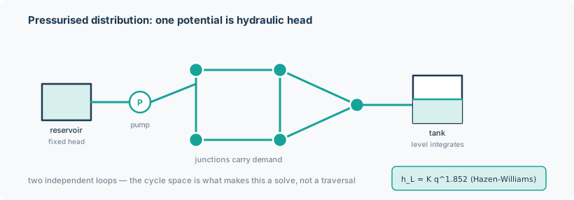
Pressurised water distribution: reservoirs and tanks at fixed or slowly varying head, and junctions with demand, are nodes; full pipes, pumps and valves are edges. Water is conserved at every junction, and flow is driven by differences in hydraulic head.

Every pipe is full and its head loss is a monotone function of the head difference, so the whole network is one KirchhoffLayer whose potential is hydraulic head. That is exactly what distinguishes it from the free-surface sewer, whose normal flow is set by slope and upstream inflow rather than by head difference.

Units. Head and elevation m, flow and demand m³/s, pressure head m (with a helper to kPa).

from noodl.apps.water import (
    Junction, Reservoir, Tank, WaterPipe, Pump, Valve, WaterNetwork, WaterOptions,
    build_model, water_steady, initial_state, twoloop,
    pressure_head, to_kilopascal, link_table, tank_inflow,
)

A reservoir and pump feeding a looped distribution network with a tank

Every type this application offers — what it does and how to call it — is listed in its catalogue. It is set up and run like every other model; see Using noodl.

A worked example¶

from noodl.apps.water import build_model, water_steady, twoloop

model, state, drivers = build_model(twoloop())
model.check(state, drivers).raise_for_errors(strict=True)
final = water_steady(model, state, drivers)

water = model.refs.water
heads = water.head.named(final[water.head])     # m, by node name
flows = water.flow.named(final[water.flow])     # m3/s, by link name
print(round(float(heads["J1"]), 6), round(float(flows["P1"]), 6))

49.267725 0.045

To change an input, give it by name over the builder's own values. A demand is a negative source (m³/s withdrawn; demand= does the sign for you), and junctions not named keep their demand. On a model built with quality= the quality sink is the withdrawal of the current hydraulic solution (a scaled or patterned water.sources, or the delivered demand under pda=True), so a tracer entering at the reservoir stays at its concentration at every demand level. A junction with a positive water.sources (an injection of water) is no sink: the injected water carries no tracer of its own and dilutes what arrives through the pipes, and any tracer injected with it is quality.sources (kg/s). On R → A → B with the reservoir at 100, an injection of 0.005 m³/s and 0.1 kg/s at A and a withdrawal of 0.01 m³/s at B, both junctions read (0.005 × 100 + 0.1) / 0.01 = 60, and the tracer withdrawn equals the tracer supplied. A STAGNANT node (no inflow and no outflow, e.g. a dead end whose delivered demand is zero under pda=True because the pressure is below the minimum) has no steady concentration without decay: water_steady raises UndefinedSteadyState naming the node and the cause, as the transport layer does for any stagnant node (a steady solve never invents a value). With a bulk decay (quality > 0) the node reads 0; or step the quality in time from an initial concentration. Quality advects through every hydraulic edge kind: pipes, pumps and valves. A pressure-driven model (pda=True) refuses both demand= and a water.sources value, since its demands are node sources set at build time:

from noodl.apps.water import initial_drivers

more = initial_drivers(model, demand={"J2": 0.012})      # m3/s withdrawn at J2
final = water_steady(model, state, more)
print(round(float(water.head.named(final[water.head])["J2"]), 6))

48.641165

In the dictionaries the heads are "water.phi" (full node order) and the flows "water.q" (link order); tank levels and pump status are the state keys "water.tank_level" and "water.link_status", set by tank and pump name with initial_state(model, values=...). See Using noodl.

twoloop() is a hand-built network: reservoir R1 at 50 m, six junctions with demands 5/8/6/10/7/9 L/s, eight Hazen-Williams pipes at \(C=130\) forming two independent loops. Its heads are 49.267731, 48.877316, 48.430882, 48.213867, 48.117119 and 48.122936 m, the same as EPANET 2.2 gives for the equivalent twoloop_si.inp.

The same network can be read from an EPANET .inp file (see File formats):

from noodl.apps.water import read_epanet_inp, build_model, water_steady

net = read_epanet_inp("twoloop_si.inp")
model, state, drivers = build_model(net)
final = water_steady(model, state, drivers)

The objects¶

Object	Fields
`Junction(name, elevation, demand=0.0, pattern=None)`	A demand node.
`Reservoir(name, head, pattern=None)`	Fixed-head boundary.
`Tank(name, elevation, init_level, min_level, max_level, diameter)`	Cylindrical tank.
`WaterPipe(name, u, v, length, diameter, roughness, minor_loss=0.0, status="OPEN")`	A full pipe.
`Pump(name, u, v, curve, power=None, speed=1.0)`	Edge oriented suction → discharge.
`Valve(name, u, v, diameter, kind, setting, minor_loss=0.0, curve=None)`	TCV, FCV, PBV or GPV (`curve`: a GPV's head-loss curve).
`WaterOptions(demand_model="DDA", minimum_pressure=0.0, required_pressure=0.1, pressure_exponent=0.5, ...)`	Carried from the file's `[OPTIONS]`.

WaterNetwork collects them plus curves, patterns, controls and the timing options. nodes() returns junctions, then reservoirs, then tanks; links() returns pipes, pumps, TCVs, FCVs, PBVs, GPVs in that order; validate() refuses anything out of scope by name.

`build_model`¶

model, state, drivers = build_model(
    net,
    headloss=None,      # 'H-W' (default) or 'D-W'; None takes the network's own
    pda=None,           # pressure-driven demand; None takes net.options
    p_min=None, p_req=None, exponent=None,
    quality=None,       # bulk decay coefficient, 1/day; adds a quality TransportLayer
    coupling="pingpong",
    dt=None,            # overrides net.hydraulic_timestep for the tank closure
    friction="composite",  # D-W friction law: 'composite' (default) or 'colebrook'
    pipe_form=None,     # 'flow' (resistance form; the default) or 'potential'
)

pipe_form is how the pipes enter the solve. In the resistance form ("flow", the default except with friction="colebrook") each pipe is dp = h(q) (FlowControlledPipe) with its flow an unknown, solved by Modified Nodal Analysis from EPANET's own first iterate (every pipe at 1 ft/s). In the potential form ("potential") each pipe's flow is the inverted law \(q = g(dp)\) on the nodal path. Both give the same solution to round-off; they differ in how Newton gets there. The potential form's slope grows without bound as a pipe's flow goes to zero, so on Net1's 24 h run the step where a control closes the pump and leaves pipe 10 dead-ended needs 136 Newton iterations; the resistance form's slope goes to EPANET's RQtol floor instead, and no step needs more than 6. The whole 24 h run over eight demand multipliers (benchmarks/water_eps.py) takes 2.5 times less time.

water_steady(model, state, drivers, **solve_kwargs) wraps model.steady with defaults atol=rtol=1e-11, max_iter=200 (both empirically tuned, the iteration cap for the potential form; caller overrides win), starts a cold start of the resistance form (every pipe flow exactly zero) from model.initial_flows, and the pumps from their design flows (EPANET's own first iterate), then checks every converged pump's flow against its own q_max() and raises naming the pump and batch instance if it is exceeded — rather than silently accepting an extrapolated point off the end of the curve.

The physics¶

Hazen-Williams¶

\[ h_L = K q^{1.852} + m q^2, \qquad K = \frac{10.666829500036\, L}{C^{1.852} d^{4.871}}, \qquad m = \frac{K_{\text{minor}}}{2 g A^2} \]

The SI constant was re-derived from EPANET's own US constant 4.727 and matches wntr's hw_k to 1.04e-9 relative. With no minor loss the inversion is closed form; with one, it is a batched monotone root solve bracketed by the pure Hazen-Williams flow as an upper bound.

Below dp_transition (default \(10^{-9}\) m) the law blends to a laminar linear form to keep the Jacobian finite. That value is empirically chosen: at 1e-9 the 24-hour tank trajectory is converged to 8.18e-5 m against EPANET, and Newton iteration counts run 50/93/136/179 at 1e-3/1e-6/1e-9/1e-12.

Darcy-Weisbach¶

CompositeDarcyWeisbach (friction="composite") is EPANET 2.2's own composite law: Hagen-Poiseuille, then Dunlop's transition cubic, then Swamee-Jain. It is transcribed from its source (hydcoeffs.c, DWpipecoeff and frictionFactor), in EPANET's internal feet and cfs:

\[ h_L = \begin{cases} (16 \pi \nu d R + m \lvert q \rvert)\, q & Re \le 2000 \quad \text{(Hagen-Poiseuille)} \\ (f(Re) R + m)\, \lvert q \rvert q & Re > 2000 \end{cases} \qquad R = \frac{L}{2 \cdot 32.2\, d A^2}, \quad m = \frac{0.02517\, K_{\text{minor}}}{d^4} \]

with \(f\) Dunlop's cubic interpolation for \(2000 < Re < 4000\) and Swamee-Jain above. The composite is \(C^1\): the cubic matches \(64/Re\) and Swamee-Jain in value and slope at its ends. EPANET's constants are kept as EPANET has them, because they are part of what it computes: \(g = 32.2\) ft/s² (not 32.174), the rounded minor-loss factor 0.02517, water at \(\nu = 1.1 \times 10^{-5}\) ft²/s times [OPTIONS] VISCOSITY, and the flow-unit factor EPANET divides a file's flows by (LPSperCFS = 28.317, GPMperCFS = 448.831, ...; WaterOptions.flow_units carries the file's unit). EPANET has no low-flow linearisation for D-W: the laminar branch is already linear through \(q = 0\), so the element needs no transition blend. The flow is found by a safeguarded Newton inversion of the odd law \(h_L(q)\) with EPANET's own analytic gradient, and differentiated by the implicit-function rule.

This is the default whenever the head loss is D-W, including every .inp read with HEADLOSS D-W, because the application's reference is EPANET. friction="colebrook" selects the framework's generic Duct instead (implicit Colebrook, a straight laminar line to its Re = 2000 value, water at \(1.002\times10^{-3}/998.2\) m²/s, standard gravity); it is a different law and does not reproduce EPANET (3.6e-4 on the two-loop heads, up to 81 % on a pipe's head loss near Re = 2000).

Pumps¶

three_point_curve(q_design, h_design) reproduces EPANET's single-point construction — shutoff head at 133% of design head, maximum flow at twice design flow — giving \(h_0 = 4H/3\), \(r = (H/3)/q_d^2\) and forcing \(n = 2\) exactly. q_max = w (h_0/r)^{1/n} is the flow at zero head gain.

Every pump enters the solve in its head-gain form, whatever the pipe_form, as EPANET and wntr write it: FlowControlledPump, \(H_{\text{discharge}} - H_{\text{suction}} = h_{\text{gain}}(q)\) with \(h_{\text{gain}} = w^2 h_0 - r w^{2-n} q^n\) and the pump's flow an unknown. Two regularisations keep the gain strictly decreasing in \(q\), so every head difference has exactly one flow:

below the flow where the curve's slope falls to EPANET's RQtol, the gain is the curve's tangent there (wntr's get_pump_line_params construction), so the slope never vanishes;
below zero flow the pump is shut: the gain rises with EPANET's closed-link slope CBIG (\(10^8\) ft/cfs). A pump held beyond its shut-off head, which EPANET closes, converges to EPANET's closed-link leak (excess head / CBIG, 3.4e-8 m³/s for 36.7 m), not to a reverse flow.

PumpCurve.flow still gives the inverted curve, \(q = w((h_0 + dp/w^2)/r)^{1/n}\), with a laminar blend near shut-off, but the solve no longer uses it: its slope is infinite at shut-off and exactly zero beyond it. A Newton iterate beyond shut-off then has no Jacobian entry between the pump's two sides, and with a pressure-driven demand downstream only the demand's own small slope ties those heads to a boundary; the next step throws them far outside the curve and the system goes singular. That was measured on a reservoir, a pump and a pipe feeding a PDA junction (singular from the fifth iterate on). In the head-gain form the pump's row ties its two heads together on every iterate, and the same network converges quadratically, in 5 Newton iterations (19 with pipe_form="potential").

Valves¶

A TCV is a settable minor loss and an FCV a fixed flow. A PBV (pressure breaker) and a GPV (general purpose valve) follow EPANET 2.2's own coefficient routines (hydcoeffs.c, pbvcoeff and gpvcoeff) as implicit laws, BreakerValve and GeneralPurposeValve, whose flow is an unknown of the layer:

PBV: the head drop from the valve's start node to its end node is its setting, whichever way the water flows. Where the open valve's minor loss \(m q^2\) exceeds the setting, or the setting is 0, it is an open valve instead, \(h = m q |q|\), with EPANET's minor-loss coefficient \(0.02517 K / d^4\) (ft, cfs) and its rounded flow-unit factor.
GPV: \(h = \operatorname{sgn}(q)\,(h_0 + r |q|)\) on the segment of its head-loss curve that brackets \(|q|\) (the first or last segment, extended, outside the curve), with \(\operatorname{sgn}(0) = +1\).

A network with either valve is solved by Modified Nodal Analysis (sparse LU); every other network stays on the nodal path. PRV and PSV, which switch status on the absolute head at one end, are not modelled.

Tanks and controls¶

TankLevels is a Model closure declaring state_keys = ("water.tank_level", "water.link_status"). Its __call__ applies controls and returns updated drivers; it does not advance the level. advance(level, inflow, dt) does that by explicit Euler, \(H \mathrel{+}= q\,\Delta t / A\). event_step(level, rate, dt) implements EPANET's adaptive step-shortening to the next control crossing.

That shortening is not optional. A fixed one-hour step was measured to diverge from EPANET by 2.07 m on Net1, because the pump switches an hour late; with event shortening the same trajectory matches to 8.181e-5 m.

An extended-period run therefore looks like this:

for _ in range(steps):
    drivers["water.sources"] = base_demand * pattern_factor(t)
    solved = water_steady(model, state, drivers)
    inflow = tank_inflow(model, solved)
    dt_eff = model.tank_closure.event_step(level, rate, dt)
    level = model.tank_closure.advance(level, inflow, dt_eff)

Tanks as storage. build_model(net, tank_mode="storage") makes every tank an interior node with a TankStorage edge to a datum node "_datum" at head 0, its level stepped implicitly inside the solve: backward Euler, \(q = A\,(H - H_{\text{prev}})/\Delta t\), or trapezoidal. water_step(model, state, drivers, dt) takes one step (Model.step, with water_steady's Newton defaults); tank_levels(model, state) reads the levels from the solved heads; the level-triggered controls stay a closure (TankStorageControls), acting on the step-start levels. The step is differentiable through time (the gradient of a level after several steps matches central differences). It is not the EPANET comparison mode: the implicit step differs from EPANET's explicit one by the step's own discretisation error. Both converge to the same trajectory, at first order: on Net1, halving the storage step halves its distance from a fine explicit run. Its event_step never shortens a step below 1 s (the implicit step lands just short of a projected crossing, and a far shorter step stalls Newton), and with steps as long as an hour a switch can land up to a step late, so sub-steps of a few minutes are the useful range. Not with quality: the combination is refused with a ValueError (a storage tank is an interior node joined to the datum by a storage edge, which the quality layer does not model as a well-mixed volume); use the default tank_mode for water quality, where a tank is a quality boundary whose concentration the caller sets. A constant tracer is preserved (every junction stays at the source concentration) across both pipe_forms, TCV, PBV and GPV valves, tanks and pda, tested in tests/apps/water.

Pressure-driven demand¶

EPANET's Wagner function (Manual eq. 13.6), with \(p = H - z\):

\[ d(p) = \begin{cases} D & p \ge P_{\text{req}} \\ D \left(\dfrac{p - P_{\min}}{P_{\text{req}} - P_{\min}}\right)^{e} & P_{\min} < p < P_{\text{req}} \\ 0 & p \le P_{\min} \end{cases} \]

Implemented with a guarded kink so both where branches stay finite and differentiable. PressureDrivenDemand refuses p_req <= p_min — a zero-span demand curve.

Verification¶

Against the real EPANET 2.2 engine through wntr 1.5.0, which bundles epanet22.dll. Note the reference implementation's own floor: EpanetSimulator reads EPANET's binary output, whose on-disk reals are float32, so roughly 1e-7 relative is EPANET's own precision, not noodl physics'.

Check	Tolerance	Measured
`twoloop_si.inp` heads and flows	rel 1e-6	4.361e-7 heads, 8.090e-8 flows
`twoloop_si.inp`, noodl physics' own nodal continuity	1e-13	2.093e-14
Net1 single period: heads, flows, pump head gain	1e-6 / 1e-5 / 1e-6	7.058e-8, 2.868e-6, 1.189e-7
Net1 24 h tank level with level-triggered pump controls	2e-4 m	8.181e-5 m worst of 25 steps
Darcy-Weisbach, `twoloop_si.inp` heads and flows	rel 1e-6	5.819e-8 heads, 6.482e-8 flows
Darcy-Weisbach, Net1 single period: heads, flows	1e-6 / 1e-5	7.009e-8, 3.986e-6
Darcy-Weisbach, laminar + transitional + turbulent pipes (`lowflow_dw_si.inp`): heads, flows, per-pipe head loss	1e-6 / 1e-6 / 2.65e-7 m	3.5e-8, 9.4e-8, 9.6e-8 m
Pressure-driven demand vs EPANET's `DEMAND MODEL PDA`	1e-5	3.521e-7 heads, 2.184e-7 demands
A pump feeding pressure-driven demand (two-loop with a pump, every junction pressure-limited), both `pipe_form`s	1e-5	3.526e-7 heads, 2.354e-7 flows, 2.355e-7 demands
PBV (active and open) and GPV on the two-loop: heads, flows, the valve's head loss	1e-6 / 1e-6 m³/s / 1e-5	5.5e-7, 2.6e-7 m³/s, 6.8e-6
Head loss sums to zero around every cycle-basis loop	1e-12	exactly 0.0
Autodiff vs central differences	1e-6 × scale	3.212e-6 / 2.505e-10 / 1.007e-6 / 2.753e-9
TRACE water quality, single source	1e-3	6.438e-12 percentage points
Golden regression	1e-10	0.0

Four rows deserve comment.

Continuity is machine-precision exact for noodl physics (2.093e-14), while EPANET itself misses continuity at Net1 node 13 by 4.5e-10 m³/s. The ~1e-7 residuals on twoloop_si.inp and the Net1 single period are attributable to EPANET's float32 output path and its own mild continuity violation, not to this solver.

Darcy-Weisbach reaches the same floor as Hazen-Williams. With EPANET's own composite law (above) the D-W rows sit at the float32 output floor. The per-pipe loss bound is derived, not fitted: EPANET stores its heads as float32 feet in its hydraulics file and reports them as float32 metres, so each reported head can be off by half a spacing in each, and a loss by twice that, \(2(0.3048 \cdot 2^{-22} + 2^{-24})\) m for heads between 1 and 2 m. Two EPANET details matter at this level: the rounded flow-unit factor (with the exact one the two-loop heads miss by 4.3e-7 instead of 5.8e-8) and, for the low-flow network, ACCURACY 1e-8 in the fixture, since at EPANET's default 1e-3 its own loop flows stop 5e-7 short of converged.

The valve row compares flows absolutely. EPANET holds an active PBV's head drop with a penalty (\(10^8\), CBIG), so its own flows are not continuous through the valve: P2 and the valve are in series through a demand-free junction, yet EPANET reports them 1.6e-7 m³/s apart, and the drop across the valve as 4.999997 m for a 5 m setting. noodl physics' flows agree to round-off and its drop is the setting.

The loop head-loss row is a formulation identity, not a comparison — head loss summing to zero around every independent loop is a property of the cycle-space formulation, and it holds exactly.

Limitations¶

Not modelled, refused by name: PRV and PSV valves; time-based controls and [RULES]; variable-speed pumps; non-cylindrical tanks; emitters; leakage; energy and cost reports; Chezy-Manning head loss; pipe-status controls and check valves. A file using any of these raises an error naming the feature.
Pump curves are single- or three-point only, with the exponent fixed at \(n = 2\). Curves with four or more points, which EPANET connects piecewise-linearly, are refused; fit a three-point curve instead.
The Colebrook option is not EPANET below Re = 4000. With friction="colebrook" a laminar D-W pipe's head loss follows a straight line to the Colebrook value at Re = 2000, not Hagen-Poiseuille, and Dunlop's transition cubic is not used. The default friction="composite" reproduces both.
Water-quality tracing is verified on a single source only. The TRACE check uses a network with one source, where the answer is 100 % everywhere it reaches; mixing of several traced sources has not been compared against EPANET.
Tank area does not enter a single water_steady call. Only the tank's head (bottom + level) enters the steady solve, so gradients with respect to tank area come from a time-stepped run (TankLevels.advance), not from the steady state.
Tank level events are not batch-safe. TankLevels.event_step indexes tanks along the first tensor dimension, so a batched (B, n_tanks) rollout with level-triggered controls gives wrong results. Run batched tank simulations one instance at a time.

Install¶

Nothing beyond the base dependencies, plus optionally sparse. wntr — the EPANET reference implementation — is test-only and deliberately not a runtime extra, because it pulls in a measured 351 MB of mandatory dependencies.

pip install "noodl-physics[dev]"     # only if you want to run the EPANET parity tests