Layers and models¶

A layer is one physical process on one network. A Model holds several layers on one network and steps them together.

This page covers the part of noodl physics least like other network solvers: there are four different ways an edge flow can be determined, and choosing the right one for your problem matters more than any other modelling decision you will make.

The four flow-determination modes¶

Most network tools support exactly one of these. noodl physics supports all four, and they compose on one graph.

#	Mode	The flow comes from	Implemented by
1	Kirchhoff solve	Both Kirchhoff laws plus the constitutive laws on the edges, solved together. Newton's method on a nodal conservation residual: \(A_I\,g(A^\top\phi) = s_I\) (with the flows of implicit constitutive laws as extra unknowns: Modified Nodal Analysis)	`KirchhoffLayer`
2	Driver-prescribed	Handed in directly as a driver value	any `TransportLayer` with no Kirchhoff-layer owner
3	Closure-computed	Computed from other state by an arbitrary function	a closure writing `"<layer>.q"`
4	Clip-and-allocate	A request, clipped against arc capacity and receiver headroom — no potential variable anywhere	`AllocatedFlowLayer`

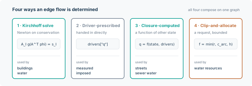
The four flow-determination modes: Kirchhoff solve, driver-prescribed, closure-computed, clip-and-allocate

Worked examples of each, from the applications:

1 — A building's airflow network. Pressures are unknown; flows follow from them.
2 — Not usually chosen alone; it is the escape hatch for a flow you measured or imposed.
3 — A street canyon. The along-canyon velocity is a closed-form function of the wind aloft and the canyon geometry, so there is no potential to solve for; StreetFlows computes every flow and writes it. The sewer's water side likewise: on a tree the cycle space is empty, so continuity alone fixes every pipe discharge in closed form.
4 — A water-resources network. An arc requests a transfer; the receiving reservoir accepts what its remaining headroom allows; the rest is unmet. There is no head, no pressure, no potential — the rule is the physics.

Getting this wrong is expensive. Modelling a gravity sewer as a potential problem, or a water-allocation rule as a pressure network, produces a model that converges to a confidently wrong answer.

`KirchhoffLayer`¶

Solves for nodal potentials such that flow is conserved at every interior node.

from noodl.layers.kirchhoff import KirchhoffLayer

layer = KirchhoffLayer(
    net,
    name="air",
    laws=[leak],                # one ConstitutiveLaw per edge kind
    drives=[stack],             # additive potential-difference terms
    boundary=["ambient"],       # nodes whose potential is prescribed
    linear_solver="auto",       # 'auto' | 'cg' | 'gmres' | 'direct' | 'sparse_direct'
    quantity="pressure",        # metadata a Model reports
    unit="Pa",
    phasor=False,               # True: complex sinusoidal steady state (see below)
)

phi, q = layer.solve(phi_boundary, drivers, sources=sources, differentiable=True)

quantity and unit are metadata only — nothing numerical reads them. They exist so that a model composing several Kirchhoff layers over one network can tell a pressure layer from a temperature one without matching on names. They are still checked for consistency: every key of a layer is a Field carrying its unit (a transport layer's unit, source_unit, capacity_unit and flow_unit give the units of its state, sources, capacity and flows), and Model.check() warns (unit-mismatch) when a closure declares a different unit for a key it reads (input_specs) or writes (output_units), and notes (unit-undeclared) a field with no unit. Units are compared as strings after trivial respelling (m3 and m^3, 1 and -); nothing is converted. See The closure contract.

Useful accessors: flows(phi, drivers) evaluates the branch law; flows_of_kind(q, kinds) extracts one kind's block from the concatenated flow vector; residual(...) and jacobian(...) expose the Newton pieces directly; kind_slice(kind) and law_for(kind) locate a kind.

diagnostics, when you pass a dict, is filled with newton_iterations, linear_iterations, method, backend, converged and residual_norm. method is what you asked for; backend is what actually ran. They are deliberately separate — see Solvers.

Modified Nodal Analysis: implicit, coupled and dynamic laws¶

A KirchhoffLayer whose constitutive laws are all potential-controlled, single-edge and static is solved by nodal analysis, as above. A layer with any law that is implicit (law_form = "implicit"), multi-port (ports > 1), dynamic or contextual, or a layer built with phasor=True, is solved by Modified Nodal Analysis instead (layer.mna is True); the declarations are described under Implicit, coupled and dynamic constitutive laws. The electrical application is built on it; the same machinery serves any domain with ideal sources, flow-controlled laws or storage on its edges.

The system. The unknowns are the interior potentials and the flows of the implicit-law edges (layer.implicit_edges, in layer edge order). The residual rows are the conservation balance at the interior nodes, \(A_I q - s_I\) (plus node sources), where \(q\) is the law's flow on a potential-controlled edge and the unknown on an implicit one, followed by every implicit law's own residual. The Jacobian is assembled as a sparse, nonsymmetric matrix from each law's local blocks (forward-mode derivatives, one per port, two on a phasor layer), so a multi-port law couples the edges of its group exactly. solve still returns (phi, q), with q covering every edge.

flows on an MNA layer. flows(phi, drivers) is a function of the potentials only on a classic layer. An implicit law's flow is not: a fan with a prescribed rise has a residual that does not contain \(q\), and conservation at the nodes fixes its flow. So an MNA layer takes the flows as input, flows(phi, drivers, q), with q as solve returned it (every edge). The implicit edges' columns are returned as given and the potential-controlled edges' columns are evaluated from phi (steady context), differentiably. At solve's own (phi, q) the result is q. Without q it raises TypeError; a phasor layer has no such accessor.

Construction checks, each raising ValueError naming the layer and the kind or nodes:

every kind's edge count is a multiple of its law's ports;
every connected part of the layer's edges contains a boundary node (a ground): a part with none (a transformer secondary left floating) has undetermined potentials;
a dynamic kind carries no drive (its step-start potential differences are taken without one);
linear_solver="cg" is refused (the system is not symmetric positive definite);
on a phasor layer, every law is phasor_capable and there are no node sources.

A system that is structurally sound but singular (a loop of ideal potential sources, a cut set of flow sources, a part reached only through flow-prescribed edges) raises a RuntimeError at the solve naming the layer and its implicit kinds. At the initial point (mode="initial") every storage law is held at its initial value and so acts as a source itself (a capacitance as a potential source, an inductance as a flow source); the error then says so and suggests starting from the operating point (mode="dc"). Under on_failure="return" that singularity shows only as converged=False in diagnostics.

The nodal-only methods (flows, dflows, residual, jacobian, linear_init, adjoint) assume every flow is a function of its own edge's potential difference and raise TypeError on such a layer; read the flows from solve's q, and the balance from balance(phi, q, sources).

The solve keywords¶

Keyword	Meaning
`mode`	`None` (default): `"transient"` when `dt` is given, `"dc"` otherwise. `"dc"`: the steady operating point (no `dt`). `"initial"`: the consistent initial point (each storage law at its initial value; no `dt`). A phasor layer is always `"phasor"`.
`dt`	One implicit step of this length (s).
`t`	The evaluation time, the END of the step on a transient (a time-dependent source is evaluated there); `None` when untracked.
`history`	`(phi, q)` at the step start, full-node potentials and every edge's flow, as `solve` returns them. Required on a step of a layer with a dynamic law.
`integration`	`"trapezoidal"` (default) or `"backward_euler"`.
`phi0`, `q0`	Warm start of the interior potentials and of the implicit-edge flows; zeros otherwise.

A layer solved by nodal analysis has static laws: it accepts t, integration, q0 and the modes "dc" and "initial" and ignores them (phi0 is its own warm start), and refuses mode="phasor", dt and history, since it takes no step. A phasor layer ignores integration and refuses dt, history and any mode but "phasor". On the differentiable path (the default) gradients reach history too, so a chain of steps back-propagates through time.

Linear solver. linear_solver="auto" on such a layer factorises: SciPy's sparse LU ("sparse_direct", per instance) whenever SciPy is importable, at any batch size, and batched dense LU ("direct") only when it is not. A dense batched factorisation costs memory and work growing with the square and cube of the system size per instance: a 64-frequency sweep of a 1604-unknown circuit took 6.1 s and 1.3 GB dense against 0.48 s with sparse LU. A tiny circuit at a very large batch may be faster with an explicit method="direct". "auto" never picks GMRES (the system is indefinite and badly scaled, with potentials and flows in one vector) and refuses CG. An explicit "gmres", "direct" or "sparse_direct" is honoured. diagnostics["method"] is the method requested and diagnostics["backend"] the one that ran.

Phasor layers¶

KirchhoffLayer(..., phasor=True) solves the sinusoidal steady state: phi, q, the boundary potentials and the warm starts are complex (complex128). The frequency in Hz comes from the driver layer.frequency_key ("<name>.frequency", one value per instance) and reaches the laws as ctx.omega = 2 pi f. Each complex unknown is solved as its (real, imaginary) pair, so a law that is not holomorphic in dp (a constant-power load, q = conj(S / dp)) is solved exactly, and the real solver machinery serves unchanged. A load is an edge to ground (node sources are refused). power_residual is then the complex power balance, real and imaginary parts both zero at a solution: Tellegen's theorem for phasors.

The initial guess is zero. A law that is singular or flat at dp = 0, such as a constant-power load, needs a warm start: pass phi0 (for example every interior potential at the nominal source voltage).

On a `Model`¶

Model gives such a layer its history, time and warm start; see Layers solved by Modified Nodal Analysis below.

`TransportLayer`¶

Advects one or more species (or heat) along the flows of its kinds, with storage at nodes:

\[ \frac{dx}{dt} = M x + N x_b + \frac{s}{\text{capacity}} \]

from noodl.layers.transport import TransportLayer

layer = TransportLayer(
    net, "thermal",
    capacity=heat_capacities,       # per ACTIVE INTERIOR node
    flow_kind=("airpath", "door"),  # one or several advecting kinds
    boundary=["ambient"],
    n_species=1,
    conduction_kind="wall",         # optional diffusive edges
    conductance=ua,
    scheme="exact",                 # 'exact' | 'implicit' | 'trapezoidal'
    quantity="temperature", unit="K",
)

Three things catch people:

The active interior. Nodes that no edge of this layer's kinds touches are inactive and have no row at all — not a zero row, which would be singular. capacity must be indexed by the active interior, which active_interior(net, kinds, boundary) computes. A wall-mass node with conduction edges and no airpath edge is an unknown of a thermal layer and is not one of a species layer over the same network.
sources is in full node order, not interior order — zeros on boundary and inactive nodes. This differs from capacity on purpose: sources are an application-level quantity, capacity a layer-level one.
flow_kind may be several kinds, and q is then their flows concatenated in that order. That is exactly what KirchhoffLayer.flows_of_kind(q, layer.flow_kinds) produces, so heat advected by both "airpath" and "door" edges needs no new operator.

The three schemes: "exact" uses an augmented matrix exponential and controls its own error by sub-stepping; "implicit" is implicit Euler; "trapezoidal" is the second-order variant. Use "exact" for heat, "implicit" for species — the application defaults reflect this.

The exact scheme bases its sub-stepping on the operator's one-norm ||dt M||_1, computed from the state-independent matrix before any arithmetic on the state; if the predicted work exceeds the budget, the step is refused, raising an error that names the layer and advises the implicit or trapezoidal schemes. A stiff operator (large ||dt M||_1, e.g. fast removal with a nonzero forcing) costs the exact scheme thousands of matvecs per step by nature; scheme="implicit" is the documented choice there, not a larger budget. All coefficients the layer owns—carrier, transmission, kinetics, removal, and conductance—are differentiable under every scheme.

Boundary values linear in time. By default, the boundary values stay constant over a step. In the exact scheme, step(..., x_boundary_end=...) instead makes them vary linearly over the step, from x_boundary at its start to x_boundary_end at its end (a first-order hold). The step is then exact for a boundary value that ramps linearly while the flows are held fixed. This matters for a zone that flushes much faster than the step. With a boundary value held at the step mean of a ramp, such a zone relaxes to that mean and ends about half a step behind the boundary. With the linear boundary, it ends behind by its own flushing time, as it should. The Modelica importer's scheme="midpoint" runner uses this. The implicit and trapezoidal schemes do not accept the argument and raise ValueError if it is given. So does step_with_transfer, which returns the boundary transfer: the transfer is defined for a boundary held constant over the step.

x_boundary_rates=(start, end), given together with x_boundary_end, adds the boundary's rates of change at both ends of the step. The boundary then follows the cubic Hermite through both ends' values and rates instead of the straight line. A fast-flushing zone ends behind its boundary by its flushing time times the boundary's rate at the step's end. On a curved boundary the straight line gets that rate wrong: it uses the chord's slope, which is off by about half a step times the curvature. The Hermite uses the end's own rate.

Changing storage. A transport layer's capacity may change over a step: a sewer pipe's wetted volume, or a headspace volume as the water level changes. The step conserves the stored amount V x in amount form: V_new x_new - V_old x_old = dt F(x_new) (implicit) or = dt/2 (F(x_new) + F(x_old)) (trapezoidal). In the trapezoidal form the old-time rate F(x_old) is evaluated with the OLD capacity, which matters for removal and kinetics (they act on the amount V x), not for advection or conduction (capacity-free amount rates). The argument capacity_prev (the storage at the step's start, when it differs from the capacity argument at the step's end) implements this; a fixed-storage layer omits both and recovers the classical form. The driver "<layer>.capacity" holds the storage at the step's end. When a closure writes that driver, the step-start state must carry the key "<layer>.capacity", the storage at the state's own time, which Model.initial_capacities(state, drivers) builds by querying the closures. The "exact" scheme has no changing-capacity form and raises by name if capacity_prev differs from capacity.

Dilution. dilution= (per species, None by default) adds dilution * net(q) / capacity to the removal, net(q) the signed net inflow of the flow edges into each node. Where the flows do not balance because the stored volume changes, dilution = carrier is the advective form V dx/dt = sum_in carrier q (x_in - x) and dilution = 0 the conservative flux form; the capacity is then a rate coefficient at the end of the step. dilution_mode="withdrawal" instead reads only max(net(q), 0): a FIXED volume whose flow imbalance is a nodal sink or source of the carrier. A surplus of inflow is a withdrawal that leaves at the node's own value; a deficit is an injection of carrier with no content of its own, which the outflow carries away, and whatever content it brings is the caller's sources, never a negative removal. The water application's quality layer uses this mode. The sink goes through torch.where, so at net(q) = 0 its derivative is the withdrawal side's. The default "signed" mode is unchanged.

Storage-free nodes. storage_free=[...] names interior nodes that hold no amount, such as a zero-volume air-handler plenum. Their balance is algebraic in every step: what flows in flows out within the step, so their value is the flow-weighted mix of what enters. A storage-free node with nothing passing through it (no flow and no conduction) keeps its value, as ContamX holds the plenum of a switched-off air handler. A source at such a node (a heating coil in a plenum) is carried on by the flow through it within the step. At a node nothing passes through the source has nowhere to go, and the step drops it (no airflow through a plenum: its coil delivers nothing); step's diagnostics reports the number of nonzero source entries dropped under "held_sources_dropped" (in Model.step, at diagnostics["layers"][name]). Their capacity, at construction or per step, may be 0 (a negative one is refused everywhere, and a zero one at any other node). Removal and kinetics act on a stored amount, so they do not act on these nodes. Only scheme="implicit" and steady can hold them: the exponential and trapezoidal steps have no algebraic form, so a layer with either scheme refuses storage-free nodes at construction. A steady solve has no value for such a node with nothing passing through it, and refuses it, naming the node. Whether such a node mixes or holds is a 0/1 choice on the flows and carries no gradient: a held node's value has zero gradient with respect to the flows, although any flow through it would switch it to mixing. layer.storage_free_mask is the (n_i,) boolean mask of these nodes.

Undefined steady states. A stored node that nothing leaves (no outflow, no conduction, no removal) keeps everything that enters it, and so does a closed group of stored nodes whose contents only circulate among themselves, never reaching a boundary outflow, a removal, a filter loss or a reaction. Their steady state is undefined without a source and unbounded with one, and the operator is singular. steady checks for this on every batch instance before it solves and raises UndefinedSteadyState (a ValueError), naming the nodes; its layer and nodes attributes say which. Step such a model through time instead, or give the nodes an exchange.

Linear solver. The "implicit" and "trapezoidal" schemes each need one linear solve per step ("exact" has none). linear_solver names it: "auto" (the default), "gmres", "gmres_jacobi", "gmres_ilu", "sparse_direct" or "direct", resolved fresh on every solve (unlike KirchhoffLayer.linear_solver, which is fixed for the layer's lifetime). "auto" picks "sparse_direct" (SciPy's sparse LU, one exact factor-and-solve, no outer iteration) at or under a batch cap of 32 instances, and plain "gmres" above it — chosen on an interleaved forward/backward benchmark across the whole family (gmres, gmres_jacobi, gmres_ilu, sparse_direct), not on iteration counts alone (benchmarks/transport_solver_bench.py). "auto" never picks gmres_jacobi/gmres_ilu: the benchmark found gmres_ilu's per-instance ILU factorisation cost (paid twice per differentiable step — once in the forward solve, once in the backward adjoint, since preconditioning is not reused across the two) the clear loser at every batch size measured, and the gmres-vs-gmres_jacobi ordering too close to the run-to-run spread to trust as a tie-break. Two fall-backs, both silent (never a raise, since "auto" is a promise to choose a backend that works): SciPy absent ("auto" would have factorised, but the optional noodl-physics[sparse] extra is not installed) falls back to gmres and warns once per process; a grad-requiring solve on the on_failure="return" early-return path (which runs outside the differentiable path's own no_grad, unlike step's ordinary forward/backward) falls back to gmres silently, since an explicit sparse_direct there would otherwise raise for a reason the caller did not ask for. diagnostics["linear"]["backend"] reports which backend actually ran on every solve.

`Reaction`¶

Applied to a transport layer's state after its step (by default), operator-split:

from noodl.layers.reaction import FirstOrderDecay

model = Model(net, layers, reactions=[("species", FirstOrderDecay(k))])

FirstOrderDecay and Photostationary (Leighton NO/NO₂/O₃) ship built in; the sewer application adds SulfideGeneration. Photostationary's default rate is evaluated at the driver "temperature" (K), which it requires by name unless a constant k_no_o3 rate overrides it.

Model(reaction_order="before_transport") applies the reactions to the step-start state before the transport step instead, so the returned state is the one after transport. The sequence of operations is the same; only the point where the state is sampled moves. The sewer application uses it because SWMM reports its water quality after mixing.

Model.steady never applies reactions. This is deliberate — a steady state under a reaction is a different fixed-point problem, not the transport steady state. The street and sewer applications each provide their own street_steady / sewer_steady helper that iterates transport and chemistry together to a joint fixed point. If you have a reaction and you call Model.steady, you get the transport-only answer.

`AllocatedFlowLayer`¶

The fourth mode. Each edge carries a requested flow; the layer clips it against arc capacity and the receiver's remaining storage headroom, sharing proportionally when several edges compete for one node's headroom.

from noodl.layers.allocation import AllocatedFlowLayer

layer = AllocatedFlowLayer(
    net, "cap", kind="link",
    s_max=storage_ceilings,   # per node, full node order; inf for unbounded
    c_arc=arc_capacities,     # per edge
    preference=weights,       # optional sharing weights, strictly positive
    mode="hard",              # 'hard' | 'smooth' | 'projection'
    n_passes=5,
)

s_new, f = layer.step(s, drivers, dt, diagnostics=diag)

In the simplest case the realised flow is just \(f = \min(r,\; c_{\text{arc}},\; h)\). The three modes differ in gradient behaviour, which is the whole reason there is more than one — see Flow allocation for the full treatment.

An allocation layer is inherently discrete-time. A Model owning one refuses a steady pass and refuses residuals() outright, because a clip-and-allocate rule has no steady meaning to report.

`Model`¶

from noodl.model import Model

model = Model(
    net,
    layers={"air": air_layer, "thermal": thermal_layer},
    closures=[density],
    reactions=[("species", decay)],
    coupling="pingpong",            # or "iterate"
    iterate_tol={"thermal": 0.01},  # REQUIRED when coupling="iterate"; transport or Kirchhoff layers
    iterate_max=20,
    substeps={"species": 4},
)

state = model.step(state, drivers, dt=60.0)
state = model.steady(state, drivers)

iterate_tol may name a transport layer (converged on its state .x) or a Kirchhoff layer (converged on the largest change of its potential .phi over its interior and boundary nodes, in the potential's units, per instance). A Kirchhoff layer is named when a closure computes that layer's element coefficients, or its boundary potentials, from its own previous solution, as the sewer dynamic wave does with its conduit coefficients and outfall heads: for example iterate_tol={"water": 1e-6} (the sewer's head layer) repeats the pass until no head moves by more than 1 micrometre. Its .phi and .q are relaxed with iterate_relaxation like a transport .x. Kirchhoff layers not named in iterate_tol are not iterated.

iterate_flow_tol={"water": 1e-9} (optional, flow units) also judges such a layer's flows: a pass converges only when its returned .q is within that of the .q it was fed. It matters when the potential solve stops on its warm start (its residual already within atol), which hands the fed potential back unchanged while the flows the closures read are still moving.

iterate_acceleration="anderson" (opt-in; default None) replaces the relaxation of those Kirchhoff layers' .phi and .q by Anderson mixing (type II, Walker & Ni 2011) over the last iterate_memory passes (default 5), and needs an iterate_flow_tol for each of them: the mixing minimises the fixed-point residual of .phi and .q, each divided by its tolerance, and the convergence test then also asks that residual of .phi to be within iterate_tol. Transport states stay relaxed. Mixing changes only the sequence of fed states, never the fixed point, and the fixed-point adjoint is unchanged. Two safeguards: an ill-conditioned history drops its oldest passes, and a mixed step that would move any entry against its own residual is replaced by the relaxed step, because the relaxed iteration only reaches fixed points that attract it and a secant step can head for one that repels it (a closure may have both; the sewer's flat, near-dry conduits do). The sewer dynamic wave builds with it and needs two to four times fewer passes.

Key conventions¶

State and driver keys are namespaced by layer name:

Key	Meaning
`"<layer>.phi"`	Nodal potentials, full node order
`"<layer>.q"`	Branch flows, the layer's kind order
`"<layer>.x"`	Transport state, interior order, `(n_i,)` or `(n_i, K)`
`"<layer>.s"`	An allocation layer's per-node storage
`"<layer>.phi_boundary"`	Prescribed boundary potentials (driver)
`"<layer>.x_boundary"`	Prescribed boundary transport state (driver)
`"<layer>.sources"`	Nodal sources, full node order (driver, optional)
`"<layer>.capacity"`	Per-step capacity override (driver, optional)
`"<layer>.removal"`	Per-step first-order removal rate, 1/s, `(n_i, K)`, replacing the layer's construction-time `removal` (driver, optional; not carried in the state, so a closure that sets it must write it every step)
`"<layer>.transmission"`	Per-step pass fraction of each flow edge, `(b_flow,)` or `(b_flow, K)` in the layer's flow order, replacing the layer's construction-time `transmission` (driver, optional; not carried in the state, so a closure that sets it must write it every step)
`"<layer>.requests"`	An allocation layer's per-edge request (driver, required)
`"<layer>.frequency"`	A phasor layer's frequency in Hz, one per instance (driver, required)

The order within a pass¶

Closures → potential solves → allocation steps → transport steps → reactions (reactions before the transport steps under reaction_order="before_transport").

The allocation step sits between the potential solves and the transport steps so that a transport layer reading "<layer>.q" sees a freshly written flow, whichever kind of layer wrote it.

Layers solved by Modified Nodal Analysis¶

A Kirchhoff layer whose constitutive laws include implicit, multi-port, dynamic or context-reading ones (layer.mna) is solved with the flows of its implicit-law edges as unknowns. Model hands such a layer what its laws need:

the warm start of those flows from "<layer>.q" in the state, when it is there;
the time the laws are evaluated at: the end of a step (t + dt for step(..., t=t)), the t of steady(..., t=t), or None when no time is given;
on a step of a layer with dynamic laws (layer.dynamic: a capacitance, an inductance), the step-start "<layer>.phi" and "<layer>.q" as its history, and dt. Both keys are then required in the state (state_from and check say so); give the first step a consistent initial point, e.g. layer.solve(..., mode="initial"). The history is always the step-start state, so coupling="iterate" re-steps every pass from the same start.

integration= ("trapezoidal" or "backward_euler") travels through **solve_kwargs; the keywords the Model sets itself (phi0, q0, history, dt, t) are refused there by name. steady solves such a layer at its operating point (a capacitance open, an inductance shorted). A layer with contextual laws but no dynamic one (a time-dependent source and resistors, no storage) takes no history: on a step it is solved at its operating point at the step end, t + dt, with ctx.mode == "dc" and ctx.dt None, which is exact for a layer that stores nothing. residuals reports layer.balance(phi, q, sources), the interior balance of the state's own flows. A phasor layer (phasor=True) has complex "<layer>.phi" and "<layer>.q" and reads the driver layer.frequency_key; the iterated coupling judges its convergence on the modulus of the change and differentiates its fixed point in the real view. Anderson mixing (iterate_acceleration="anderson") is refused on a phasor layer. line_search="convex" (by keyword or through newton_defaults) is refused on such a layer: its residual is not the gradient of a convex function. analytic_primal has no effect on it, because its solve already assembles the analytic operator.

Closures¶

A closure is (state, drivers) -> driver updates. It is the escape hatch for anything that is a function of solved state: air density from temperature, canyon velocities from wind, tank levels from the previous step.

def density(state, drivers):
    T = state["thermal.x"]
    return {"rho": P_REF / (R_AIR * T)}

Closures may not write layer state keys. A closure may carry its own state across steps by declaring state_keys, which Model copies from its return into the returned state — a sewer manhole level, or a water tank level and its controlled links' status. Two closures claiming one key is refused at construction, naming both, rather than resolved by whichever ran last.

Closures and the clock¶

A closure that only computes coefficients or forcing terms keeps the two-argument form closure(state, drivers). A closure that integrates some state over the step (such as a storage sweep that advances manhole levels) declares integrates = True and receives a third argument, ctx = StepContext(dt, t), where dt is the integration interval and t the step's start time if tracked. Inside step(...) the context carries the interval; inside steady(...) it refuses the closure by name because there is no interval to integrate over. Queries (residuals, current_flows, and the sewer report) call closures with ctx = None, where an integrating closure evaluates its outputs at the given state without advancing it. A closure declaring state_keys must also declare integrates (True or False) so the model knows whether its carried state changes step to step; omitting it is refused by name.

What a closure may declare¶

Everything a closure says about itself is an optional attribute, listed in noodl.contracts.CLOSURE_ATTRIBUTES and read once, at construction, into a ClosureSpec (integrates, state_keys, inputs, outputs, input_specs, key_labels, edge_kinds, requires_coupling, reads_flows_of, species_columns). A malformed declaration is refused at construction by name:

inputs, outputs, state_keys and edge_kinds must be tuples of names; a bare string (outputs = "rho") is a TypeError;
integrates must be True or False;
a declared output may not be a layer's state key ("<layer>.phi", .q, .x, .s), apart from "<layer>.q" of a transport layer no Kirchhoff layer owns;
species_columns = {layer: {species: column}}, for a closure or reaction that addresses species by column index, must agree with the layer's species_names and n_species.

model.refs.ownership() lists, for every key, who writes it and who reads it (layers, closures by their declarations, the caller); model.check reports closures that overwrite each other's declared outputs (overwritten-output), declare nothing (undeclared-closure), return keys they did not declare when probed (declared-vs-probed), or declare a unit that differs from the field's (unit-mismatch, with unit-undeclared for a field with no unit).

The two couplings, and the trap in the default¶

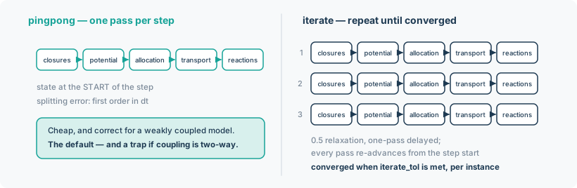
Ping-pong takes one pass per step; iterate repeats the pass until the named states stop changing

coupling="pingpong" (the default) takes exactly one pass per step, with the state at the start of the step. It is cheap, it is what a weakly coupled model wants, and its splitting error is first order in dt.

coupling="iterate" — Hensen's "onion" — repeats that pass within the one step until the transport states named in iterate_tol stop changing, at most iterate_max times. Successive substitution with 0.5 relaxation, applied with a one-pass delay: pass 1 sees the step-start state, pass 2 sees pass 1's transport states unrelaxed, and from pass 3 on each pass sees the mean of the two before it. Every pass re-advances from the step-start state, so passes never compound into passes × dt.

The trap. Calling .steady() at the defaults on a two-way coupled model solves the airflow at the temperatures the closures saw — the initial ones — and never re-converges it against the temperatures it produced. It does not warn you; it returns a plausible number. Whenever the flow depends on what it carries, pass coupling="iterate" with an iterate_tol.

Three more things about iterate_tol:

It is absolute, in each layer's own units. A species layer whose mass fractions are \(\sim10^{-3}\) and a thermal layer in kelvin cannot share a tolerance, which is why it is a per-layer mapping. A transport layer left out of it is stepped every pass but not tested.
It has a floor: the potential solve's own residual, propagated through \(dT/dF\). A tolerance tighter than that can never be met, and the run raises naming the layer, the change and the tolerance. A tight iterate_tol needs a matching atol/rtol on the step/steady call.
Convergence is decided per batch instance. A batch that fails raises naming the instances; on_failure="return" with a diagnostics dict returns instead of raising.
A pass is one iterate. A potential solve that does not converge within a pass hands back its last Newton iterate and the iteration carries on from it (that pass is never judged converged); only the iteration's own verdict raises. A solve that is differentiated still raises (on_failure="return_primal", the passes' default), and an explicit on_failure is passed through as given.

Introspection¶

model.residuals(state, drivers)   # per-layer nodal balance residual
model.ports(state)                 # what a coupled or external model may prescribe and read

Ports reports boundary nodes, prescribable keys, boundary flows, and each transport layer's flow driver key. Model.flow_layer_of[name] is None tells you whether a transport layer's flows are yours to prescribe. This is the surface the coupling application builds on.

Differentiability¶

Ping-pong is one pass of differentiable operations. Iterate runs its passes to convergence without a graph, then re-runs the certified pass once more on the graph and attaches the implicit adjoint of the interface equations — memory is one pass, not all of them, and the gradient error is of the order of the primal residual rather than tied to the pass count. The convergence decision is still made on detached copies, so it never appears in the graph. See Differentiability and Coupling for the full contract. **solve_kwargs on step/steady reach the potential solves only (differentiable, on_failure, method, Newton options); transport steps always raise on failure.