Concepts

noodl physics is built from seven ideas that stack. Each section below is a page; read them in order the first time.

Page	What it covers
Networks	Network: the typed multigraph, its incidence and cycle operators, boundary and interior, batching.
Components	Subnetworks with ports, connect, flatten() to one network, dotted names, placement, shared nodes, and reading results by component.
Constitutive laws and drives	The constitutive laws on edges, and the driving terms added to potential differences.
Layers and models	The four ways a flow is determined, the layer types that implement them, and Model, which steps several together.
Using noodl	The one way every model is used: configure, initialise by name, check, run; the parts every model shares; node orders and the setup report.
Solvers	The matvec-free linear-operator contract, Newton, and how method="auto" chooses a backend.
Differentiability	What gradients flow through, the adjoint, and the contract your laws must satisfy.
Mutation, devices and serialization	What may change after construction, how a model is moved, and what copying and saving keep.

The shape of a model

Every noodl physics model is the same four-part object, whatever the physics:

Network            a typed multigraph: nodes hold storage, edges carry flow
  |
  +-- Laws         the constitutive law on each edge kind
  +-- Drives       terms added to the potential difference (stack, wind, drag)
  +-- Closures     arbitrary functions of state that produce driver values
  |
Layers             Kirchhoff, transport, reaction, flow allocation
  |
Model              several layers on one network, stepped together

Read it bottom-up and it is a simulator. Read it top-down and it is a factorisation: the framework owns the graph, the conservation law and the solve; your problem owns the constitutive laws, the drives and the closures. Everything domain-specific in the seven applications lives in those last three boxes.

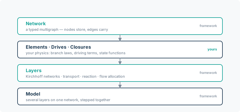
The central claim

A node conserves. An edge constitutes. That separation is what lets one piece of machinery carry a building's pressure network and a sewer's headspace air.

Concretely, a Kirchhoff layer assembles and solves

\[ A_I \, g\!\left(A^{\top}\phi + \text{drive};\ \theta\right) - s_I = 0 \]

where \(A\) is the network's incidence matrix, \(A_I\) its interior rows, \(g\) the stack of element laws, \(\phi\) the nodal potentials, \(\theta\) the element parameters and \(s_I\) the nodal sources. The framework supplies \(A\), the Newton solve and the adjoint. You supply \(g\).

Storage and transport add time: nodes accumulate, edges advect what the flows carry. The same incidence structure serves both, which is why heat riding on an airflow needs no new operator — only the flows of the kinds it advects on.

What noodl physics does not decide for you

Three choices are deliberately left in your hands, and each has bitten someone:

• How a flow is determined. A Kirchhoff solve is one of four options, not the default answer. A sewer's tree flow comes from continuity, a street's from a closure, a water-resources arc's from a clipped request. See Layers and models.
• How tightly coupled layers must agree. coupling="pingpong" takes one pass and is first-order accurate in dt; coupling="iterate" iterates to a tolerance you set. The default is the cheap one, which is wrong for a strongly two-way coupled model.
• Which linear backend runs. method="auto" picks on measured evidence, but an explicit choice is always honoured.