Coupling¶

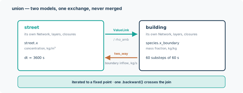
Two physical systems that meet at a shared boundary, each modelled as its own network: a street canyon and a building ventilated from it, for example, where infiltration draws the street's polluted air into the building and the building acts as a sink on the street. Each model conserves its own quantities on its own graph; at the boundary they exchange named values each step (a concentration one way, a mass flux in kg/s the other), iterated to a fixed point, so that what one side loses the other gains. The join is differentiable: gradients flow across it as if the two models were one.

Two levels of coupling¶

These are easy to confuse, and they solve different problems.

Within one model. Several physics layers on one Network inside a single Model, stepped together under coupling="pingpong" or coupling="iterate". A building's airflow and its heat balance are coupled this way: one graph, one model, several layers. See Layers and models.

Across two models. Two separately built Model objects, each with its own Network, its own layers and its own closures, coupled by union. A street network and a building are coupled this way: two graphs that were never meant to be one.

This page is about the second.

from noodl.couple import union, ValueLink, DriverAlias

What `union` does — and deliberately does not¶

union exchanges named driver and state values between two ordinary Model.step calls each outer step, iterating to a fixed point when a link is two-way.

It never merges the networks, never rebuilds the layers, and never reconstructs the closures. That is a hard constraint, not an optimisation.

The reason is closures. Layers are reconstructible from standard arguments, but a closure is an arbitrary application object — StreetFlows, a building's density closure — bound at construction time to one specific Network with application-specific constructor arguments that domain-agnostic code cannot know. Rebuilding them generically would require the coupling module to import application internals, which would break the "neither model is modified" guarantee as thoroughly as editing the application itself.

So noodl/couple.py never imports from noodl.apps.*. It reads and writes named keys and applies registered unit conversions, and it never inspects any application's internals. That is what lets the same machinery couple any pair of models, regardless of which layer type produces which flow.

Each model's own step call stays an ordinary, unmodified call. And because PyTorch's autograd tracks the computation graph rather than Python object structure, gradients cross the join in one .backward() exactly as if the two models were one object.

After a union, the original models still run standalone, bit-for-bit identical — which is pinned by a test.

Two independent models exchanging values through a ValueLink, iterated to a fixed point

A worked example¶

import torch
from noodl.couple import ValueLink, union

link = ValueLink(
    from_model="street", from_key="street.x", from_index=0,
    to_model="building", to_key="species.x_boundary", to_index=0,
    convert="concentration_to_mass_fraction",
)

coupled_model, state, drivers = union(
    {
        "street": (street_model, street_state, street_drivers),
        "building": (building_model, building_state, building_drivers),
    },
    shared=[link],
)

new_state = coupled_model.step(state, drivers, dt=1.0)

With street.x[0] = 3.0 kg/m³ and the building's rho_amb = 1.2, the building sees a boundary mass fraction of \(3.0 / 1.2 = 2.5\) kg/kg for that step.

(Condensed from tests/test_couple.py. Each model is built in the ordinary way; the full demo in tests/verification/test_coupling_demo.py puts a CONTAM .prj building on a small synthetic street network and is longer only because of the wiring, not the coupling API.)

The API¶

`union`¶

union(
    models,                # {tag: (Model, State, Drivers)}
    shared,                # a flat sequence of ValueLink and DriverAlias
    *,
    substeps=None,         # {tag: k} — step this model k times per outer step
    relaxation=0.5,
    iterate_rtol=1e-8,
    iterate_atol=0.0,
    iterate_max=50,
    adjoint_rtol=1e-10,    # tolerance of the implicit adjoint solve, not of the primal
) -> (CoupledModel, {tag: State}, {tag: Drivers})

The (Model, State, Drivers) triple is exactly what street_aq.build_model, project_to_model, sewer.build_model, water.build_model and electrical.build_model all return. union returns fresh copies and never mutates its inputs.

Two-wayness is set per link through ValueLink.two_way, not by an argument to union.

`CoupledModel.step`¶

coupled_model.step(state, drivers, dt, *, t=None, diagnostics=None)  # -> {tag: State}

t (s) is the simulation time at the start of the step, exactly as Model.step takes it, and is forwarded to every model: a time-dependent law (a ramp or pulse source) and an integrating closure see the coupled model's clock. A model with substeps={tag: k} runs its i-th sub-step of dt/k from t + i·dt/k. Every pass of the two-way iteration re-steps the same interval [t, t + dt] from the step-start state, so the clock never advances with the pass count. Without t, a model sees no clock, as with Model.step, and a time-dependent law refuses to evaluate.

`ValueLink`¶

ValueLink(
    from_model, from_key, from_index,
    to_model, to_key, to_index=0,
    convert=None,          # a registered conversion name, applied forward
    two_way=False,
    convert_back=None,     # applied to the feedback flux
    sources_key=None,      # defaults to "<from layer>.sources"
)

from_key is a transport layer's state key "<layer>.x"; from_index a position on that layer's active interior axis.
to_key must be a transport layer's boundary driver "<layer>.x_boundary" — enforced at construction, raising if not; to_index a position on the boundary axis.
sources_key, if given, must end .sources.
The two-way feedback is added to the source term, never overwritten — so a lateral load already in sources survives.

One-way link timing has a subtlety. In a union with no two-way link, the single pass reads the forward value from the step-start state — explicit ping-pong. In a union that also has a two-way link, every pass, one-way links included, reads from the previous pass's output, so a one-way link there carries an end-of-step value. One-way links are never part of the convergence test.

`DriverAlias`¶

DriverAlias(
    source=("street", "theta_w"),
    targets=(("building", "theta_w", "math_rad_to_compass_deg"),),
)

The source is authoritative; every target driver is overwritten from it through its own conversion. Applied once per step, before any pass — drivers do not change between passes, only glue values derived from state do.

Helpers¶

apply_conversion(name, value, drivers) applies a registered conversion, returning value unchanged for None and raising with the sorted list of registered names for an unknown one — an unregistered conversion is never silently treated as identity.

transport_boundary_inflow(...) returns the net mass inflow at a boundary node of a transport layer, computed from a single state snapshot. Model.ports() cannot supply this: it reports boundary_flows for potential layers only. The coupler builds the two-way feedback through differentiate_fixed_point instead (see "The fixed point" below); transport_boundary_inflow is kept as a public helper and used in tests as an independent hand reconstruction.

Unit conversions¶

Name	Formula
`concentration_to_mass_fraction`	\(x = c / \rho_{\text{amb}}\)
`mass_fraction_to_concentration`	\(c = x \cdot \rho_{\text{amb}}\)
`math_rad_to_compass_deg`	\(W_d = (270° - \deg\theta) \bmod 360°\)
`compass_deg_to_math_rad`	\(\theta = \big(\mathrm{rad}(270° - W_d)\big) \bmod 2\pi\)

The density pair is a genuine unit mismatch, not a scale factor: the street application's transport state is a concentration in kg/m³, while CONTAM's species convention is a mass fraction in kg/kg, and the two are related by the local air density.

The wind-direction pair exists because the two conventions differ in both origin and sense. CONTAM's \(W_d\) is degrees clockwise from north, giving the direction the wind blows from. The street application's \(\theta_w\) is radians counter-clockwise from east, giving the direction it blows toward. A west wind is \(W_d = 270°\) and \(\theta = 0\); a north wind is \(W_d = 0°\) and \(\theta = 3\pi/2\). Both are pinned on the cardinal points by test.

Note that the backward link in the canonical pairing needs convert_back=None: the feedback is the recipient's own integrated boundary transfer (an amount, divided by dt into a rate), a mass flux in kg/s on both sides already.

The fixed point¶

When any link is two-way, step routes through the iteration, on a recipient-first Gauss-Seidel schedule: the model that a two-way link writes its forward value into — the recipient — is stepped before its donor, and the donor receives exactly the amount the recipient's own step integrated across the shared boundary, never a flux recomputed from a state that has not been stepped yet.

Apply the one-way links from the latest state (the previous pass's output, or the step-start state on the first pass).
For each two-way link, compute the raw forward value from the latest state, relax it against the previous pass's value, and write it onto the recipient's boundary driver.
Step every recipient once, from the step-start state — never from the previous pass's output — recording the boundary transfer Model.step integrated over the recipient's own whole outer step (its sub-steps included).
For each two-way link, divide that integrated transfer by dt and add it, as a source rate, into the donor's sources, for the donor's own whole outer step.
Step every other model (donors and any uncoupled models) once, from the step-start state.
Test convergence.

Step 3's "from the step-start state" is what keeps the scheme correct: passes never compound into passes × dt. Because the donor is always given exactly what the recipient's own scheme integrated this same pass, conservation holds on every returned pass, not only at convergence — no separate residual is needed to enforce it (independently checked in tests/test_couple_conservation.py, closed exchanges to floating-point precision regardless of scheme or sub-step ratio).

Convergence is judged on the unrelaxed residual of the fixed-point map, \(\lvert g(v_k) - v_k \rvert \le \text{atol} + \text{rtol}\,\lvert g(v_k) \rvert\) — the returned forward value \(g(v_k)\), recomputed from this pass's own output state, against \(v_k\), the relaxed value the recipient was actually stepped with in this same pass — per link and per batch instance, inside no_grad, on every pass including the first. Judging the relaxed increment that produced \(v_k\) instead would make the effective tolerance scale with the relaxation factor, letting a heavily damped run falsely report convergence while \(g(v_k)\) still disagrees with \(v_k\) by a large, unrelaxed amount.

A model that is both a recipient and a donor of two-way links is refused at construction: the recipient-first schedule has no defined order for a cycle of two-way links.

Failure to converge in iterate_max passes raises naming the link — for example "street:street.x[0]->building:species.x_boundary" — the failing instances, and the largest change.

With diagnostics, you get {"passes", "converged", "max_change", "transfers", "adjoint", "adjoint_batched"} — transfers is the recipient's own integrated transfer per two-way link, from the pass that produced the returned state, keyed the same way as max_change; passes counts primal passes; adjoint is "implicit" when the returned state carries the fixed point's adjoint and None when nothing differentiable reached it; adjoint_batched says whether the adjoint was solved per batch instance (True) or across the whole batch as one system (False, also when no adjoint was attached; see Limitations). Every value in the dict is detached: diagnostics are a report, and a transfer still attached to the pass graph would offer a silent route around the adjoint.

Differentiating the fixed point¶

The passes of the iteration carry no autograd graph. Once the interface has converged, the certified pass is run once more on the graph at the same interface values — reproducing it to solver accuracy — and solvers.fixed_point.differentiate_fixed_point attaches the implicit adjoint of the interface equations to it. Writing \(y = S(z^*, \theta)\) for that pass's whole output and \(G\) for the map that reads the next iterate out of it, the returned gradient is

\[ \frac{\partial y}{\partial \theta} = S_\theta + S_z (I - G_z)^{-1} G_\theta, \]

obtained from one small GMRES solve (adjoint_rtol) whose matvec is a VJP through that single pass. Three consequences:

the gradient is the converged interface's, not the truncated iteration's. Its error is of the order of the primal residual, rather than the unrolled \(O(\rho^{\text{passes}})\) counted from the start state — an error tied to nothing the caller controls, and worst exactly where the primal is cheapest. Where the interface equations are linear in the interface the adjoint is exact whatever the residual, which is why the linear two-model test fixtures return \(1/3\) and \(2/3\) to one ulp at iterate_rtol \(10^{-12}\) and \(10^{-3}\) alike;
backward memory is one pass, not all of them;
whether anything differentiable reaches the state cannot be read off the states and drivers (a parameter may be captured inside a model's own closure), so it is asked by running a pass on the graph and dropping that graph. Pass 1 asks first; when it finds nothing, the question is asked once more at the certified interface, because a closure may take a parameter-dependent branch only after the coupled values have moved — the answer that counts is the one at the point whose derivative is returned. That extra pass (not counted in passes) is paid on every converged step run with grad mode on, because no inspection of the models can prove that nothing a pass reads requires grad (a closure may read a tensor through a module attribute, a global or a captured cell). It is skipped under torch.no_grad(), so a forward-only simulation should run under torch.no_grad(): it then pays neither the probe pass nor pass 1's graph.

The interface is every link's forward value, one-way links included, because that is what a pass reads from the previous pass's output. Only the two-way entries are measured for convergence — only they close a loop that can fail to converge.

"Reproducing it to solver accuracy" is deliberate wording: the extra pass is the same function of the same arguments, but solvers/select.py drops the SuperLU fast path for an input that requires grad, so it can take a different linear-solver route than the primal passes did. It came out bitwise identical on every fixture measured, and conservation does not depend on it either way — that is a property of the pass itself, not of which solver ran inside it.

The canonical pairing: street ↔ building¶

Forward, converted: the street's segment concentration street.x[i] becomes the building's species.x_boundary, divided by the building's own rho_amb. When a closure of the building model computes rho_amb (its density closure, from the node temperatures a schedule or a weather file sets), the coupler takes that closure's value at the start of each step, not the value the drivers were built with. An integrating density closure is called there with the step's clock (start time t, and the building's own step dt / k under substeps), so a density that follows t converts at the step-start time.
Backward, two-way, unconverted: the building is the recipient, so it is stepped first, from that boundary value; its own species boundary transfer, integrated over its whole outer step, divided by dt, is added into street.sources at the shared segment — already a mass flux in kg/s on both sides, so no conversion is needed.
Aliased weather drivers: the street's U_ref → the building's V_met with no conversion (the street is built at \(z_{\text{ref}} = 10\) m, matching CONTAM's met-station convention), and theta_w → theta_w through the wind-direction conversion.
Multi-rate: substeps={"building": 60} — the street steps once per hour, the building sixty times at 60 s, with the glue-derived boundary held constant across the inner steps. That is an accuracy simplification, not a conservation one, and it is conservative regardless: whatever the building actually integrates across those sixty sub-steps — with the boundary held constant or interpolated — is exactly the amount reported back and added to the street's sources, so holding it constant cannot leak or fabricate mass, only make the building's own response to a changing boundary less accurate within the hour.

Physically, infiltration draws segment air into the building and the building acts as a sink on the street side. Both demos assert that sign.

Verification¶

Check	Tolerance	Measured
The returned state's forward value agrees with the value the recipient was stepped with, to rtol	rtol 1e-9, atol 1e-14	holds
Gradient across the join vs central differences	rel 1e-5	holds
`substeps={"building": k}` calls the fast model exactly `k` times per slow step	exact	holds
Closed two-way exchange conserves the total amount — exact/implicit/trapezoidal schemes, 1 and 4 recipient sub-steps	abs 1e-10	holds
2×2 analytic fixed point (one implicit step each, unit source into the recipient) solves to \((4/3, 5/3)\)	abs 1e-9	holds
Structural guard: a two-way step assembles no dense topology operator (`upwind`/`incidence`/selectors)	n/a	holds
Synthetic back-coupling, 2×3 m canyon: one-way 4.169740e-08 vs two-way 4.145151e-08 kg/m³	measured	0.5897 % change, 27 passes
Loose sequential file exchange vs the two-way result	measured	0.5897 % discrepancy — equal to the street-side change, as expected for a boundary response linear in the shared value
Leakage calibration through the join	rel err < 0.05	1.288e-4, final loss 3.4574e-08
Source attribution by one adjoint pass vs central differences	rel 1e-4	1.3e-8, 2.0e-9; third source structurally zero
One measured path recovers all four branch flows	rtol 1e-10	exact

The synthetic case is deliberately sized so that the building matters: a 2×3 m canyon, where the building's infiltration changes the street concentration by 0.5897 %. On a street of realistic size one building's infiltration changes the street's concentration very little, and the coupled result should be read with that in mind.

Performance. The street ↔ building demo (benchmarks/coupling_street_building.py) couples 6 hours with 60 building sub-steps per street hour. On one workstation it took about 55 s at batch 1, 48 s at batch 10 and 137 s at batch 100 (medians; wall time varied by up to about 20 s between repeats, while pass counts did not vary at all). Three things set the cost:

Outer passes. The run needs 107 passes at batch 1 and 118 at batches 10 and 100: a batch is converged only when every instance is, so a batch spanning a wider range of conditions (here wind speeds of 1–4 m/s rather than 1 m/s alone) takes as many passes as its slowest instance.
Batch size. Cost grows far more slowly than the batch: 100 instances cost about 2.5 times one instance. Batching many scenarios into one run is much cheaper than running them one by one.
Boundary transfers. A two-way link reads the recipient's boundary transfer, which costs more than a plain step. union requests it only from the linked transport layers, so an unlinked layer on the recipient (a thermal layer, say) takes the cheaper plain step; there is nothing to set.

Limitations¶

No steady solve. CoupledModel steps in time only; there is no CoupledModel.steady. To reach a coupled steady state, step until the interface values stop changing.
Fixed relaxation. Each step is iterated with a constant relaxation factor (relaxation, default 0.5); there is no adaptive scheme. The demo fixtures converge in 21–27 passes to rtol \(10^{-10}\). Where the coupled problem has several fixed points, a constant relaxation can settle on the wrong one or fail to hold an unstable one — the same behaviour as the building application's three-steady-state case. Check a suspect result against a smaller relaxation or a different starting state.
Two-way links carry a single species on a single flow kind. A two-way link is refused at construction (ValueError) unless both layers have n_species == 1 and the recipient's layer has exactly one flow kind. Couple several species with one-way links, or one model per species.
No cycles of two-way links. Each two-way link is solved recipient first, so a model that is both a recipient and a donor of two-way links is refused at construction, with an error naming it.
One-way links are not in the convergence test. Only two-way interface values are checked for convergence. A one-way value is passed on from the previous pass and is as converged as the state it is read from — which is also the state step returns.
Three-way unions are untested. union has been verified on two-model pairings (street ↔ building above). A three-model union such as sewer + street + building is expected to work but has not been built or tested.
Only noodl physics models can be coupled. union joins noodl physics Models. There is no co-simulation interface to non-differentiable tools such as EnergyPlus or WSIMOD itself.
Ambient temperature is not coupled in the street ↔ building demo. The building sees the street only through species concentrations; its ambient density comes from the .prj file's own outdoor temperature, and the street model's drivers carry no temperature.
Batched gradients. When every interface value carries the batch dimension, the adjoint solves each batch instance independently and its cost does not grow with the batch size. A value shared across instances couples them, and the adjoint then solves the whole batch as one system, which can cost up to B times as much for B instances.