Differentiability

Every quantity in noodl physics is a PyTorch tensor and every solve is differentiable. This is the difference between a simulator and a tool you can calibrate, invert and optimise with.

What you get

For a converged solve, gradients flow back to:

• phi_boundary and x_boundary — the prescribed boundary values,
• sources — the nodal source terms,
• every value in the drivers mapping,
• every law parameter registered with learnable=True,
• and, across a coupled model, through the join into the other model's parameters.

phi, q = layer.solve(phi_boundary, drivers, sources=sources)   # differentiable=True default
loss = (phi[room] - measured) ** 2
loss.backward()

The adjoint, not an unrolled tape

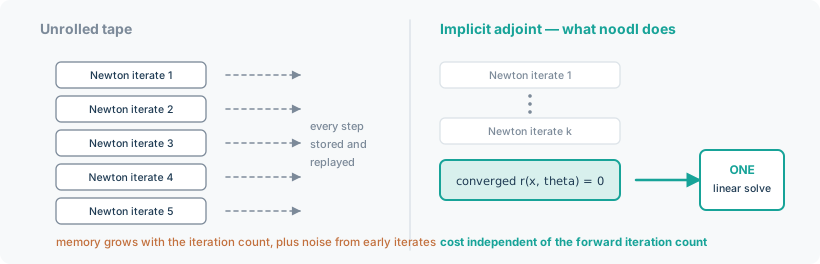
The naive way to differentiate a Newton solve is to record every iteration and back-propagate through all of them. That costs memory proportional to the iteration count and is numerically noisy — the early iterates are far from the solution and contribute derivative noise.

noodl physics does not do that. It applies the implicit-function theorem at the converged solution. For a residual \(r(x, \theta) = 0\),

\[ \frac{\partial x}{\partial \theta} = -\left(\frac{\partial r}{\partial x}\right)^{-1} \frac{\partial r}{\partial \theta} \]

so the backward pass is one transposed linear solve, whatever the forward took. The Jacobian is the one Newton already assembled, and the transposed solve reuses the same operator through TransposeOperator. For a symmetric operator — which a Kirchhoff layer's is — rmatvec is the forward action, so nothing extra is built.

The practical consequence: a model that takes 12 Newton iterations to converge costs the same to differentiate as one that takes 3.

The exception is iteration at the Model level — and it is not an unrolled exception. coupling="iterate" and CoupledModel's two-way fixed point both run their passes to convergence without a graph, run the certified pass once more on the graph at the converged interface, and attach the implicit adjoint of the interface equations (solvers.fixed_point.differentiate_fixed_point): one small GMRES solve at the converged interface, backward memory is one pass, and the gradient error is of the order of the primal residual rather than the unrolled truncation counted from the start state. The convergence decision itself is still made on detached copies and never enters the graph.

The contract

For differentiable=True to be safe, two rules must hold. A violation raises a ValueError — naming the offending law or drive and the attribute where it can — rather than silently returning a wrong or absent gradient.

The differentiable solve threads a fixed set of tensors through Function.apply: each law's and node source's registered parameters, the driver values, sources and the boundary potentials (and, on a transient step, the step-start state). Any other tensor that requires grad and reaches the residual is invisible to the implicit adjoint. Two checks look for one:

• Before solving, by attribute. Every tensor a law, node source or drive holds — plain attributes, registered buffers, and tensors nested in lists, tuples, dicts, sets and plain objects — is scanned, and one that requires grad without being threaded is refused by name.
• At the starting guess and again at the root, by evaluation. The layer evaluates its residual with every threaded tensor detached; if the result still requires grad, some other tensor reaches it (a tensor captured by a closure, which no scan can see), and the solve is refused. The root is the point the adjoint linearises at, so a law that reads such a tensor only on a branch the solve reaches after leaving the starting guess is caught there. Each evaluation costs one residual evaluation.

What the evaluation establishes is structural and pointwise: the residual's autograd graph at those two points reaches no un-threaded tensor. It does not prove that no such tensor could be read elsewhere in the state space, and it does not inspect a tensor that requires grad but is not used at the root; neither affects the gradient at the returned solution. (The Jacobian is the autograd derivative of the same flows, so it reads nothing the residual does not.)

1. A law's differentiable state must be a registered parameter.

leak = PowerLaw(C=torch.tensor(0.01), n=torch.tensor(0.65), learnable=True)   # correct

A bare tensor held with requires_grad=True outside named_parameters() is a supported construction, and its graph is reachable through the law's own component calls — but it is invisible to the differentiable solve. Since differentiable=False returns detached tensors, neither path would carry a gradient to it. Only a registered parameter is reachable, so a gradient-carrying tensor anywhere else — a plain attribute, a registered buffer, a tensor in a list, dict or plain object, the parameter of a module kept in a plain Python list — is refused. The attribute scan walks what the law holds (attributes, buffers, and containers and plain objects nested up to eight levels, skipping containers of more than 1024 items); a tensor it does not reach is caught by the residual evaluation where the residual reads it.

2. A drive must read every differentiable quantity from the drivers mapping, never hold one as an instance attribute. See Constitutive laws and drives for why this is structural rather than stylistic.

What is guaranteed

The sections above describe how noodl physics differentiates and what it takes to keep that safe. This section states the contract itself, as a list of bounded claims, each pinned to the test that would fail if the claim stopped holding.

• First-order derivatives only. The implicit adjoint never builds a graph connecting its own returned gradients back to its inputs, so a second torch.autograd.grad(..., create_graph=True) through an already-differentiated implicit solve is refused by name, inside backward() at the moment that second differentiation is attempted, rather than silently returning an incomplete result with a missing second-order term (pinned by tests/solvers/test_implicit.py::test_second_order_differentiation_raises_instead_of_silently_dropping_a_term).
• At regular solutions. The guarantee above is for a converged solve at which the residual's Jacobian is invertible; every implicit-adjoint gradient this page cites is checked at such a point, both for a linear system and for a Newton solve of a nonlinear one (pinned by tests/solvers/test_implicit.py::test_gradcheck_implicit_solve_batched_wrt_linear_system_matrix_entries and tests/solvers/test_implicit.py::test_gradcheck_implicit_solve_on_cube_root_wrt_parameter).
• Implicit adjoint for linear and Newton solves. For a residual \(R(z, \theta) = 0\) solved at \(z^*\), the backward pass solves the transposed system for the adjoint variable, \(R_z^T \lambda = L_z\), and then assembles the parameter gradient from one more pass through the residual, \(dL/d\theta = L_\theta - R_\theta^T \lambda\) — never by unrolling the forward iteration. adjoint() solving the transposed system is checked directly (pinned by tests/solvers/test_implicit.py::test_adjoint_solves_the_transposed_system), and the same construction is what _LinearSolve in noodl.layers.transport specialises to a linear residual (its own class docstring calls out solvers/implicit.py's warning "almost verbatim, because it is the identical trap").
• A discrete-step derivative for every integrator, including the exponential action with a state-independent term count. implicit, trapezoidal and exact (matrix-exponential) schemes are all differentiable, and the exact scheme's tangent at equilibrium matches the analytic matrix-exponential derivative even from \(x_0 = 0\) or \(x_0 \to 0\), because the Taylor schedule (substep count \(s\), term count \(m\)) is computed from \(\lVert dt\, M\rVert_1\) under no_grad before any arithmetic on \(x\) or the forcing term runs, and bounds the truncation of both the state polynomial and the forcing polynomial together with each one's own derivative with respect to the operator -- on the forcing (affine) path AND on the shifted (homogeneous) path a sealed pure-decay zone takes -- so coefficient sensitivities are accurate at and near a zero operator on both paths, not just the forward value (pinned by tests/layers/test_transport_derivatives.py::test_exact_step_tangent_matches_the_matrix_exponential_at_equilibrium, tests/layers/test_expm_schedule.py::test_forced_step_value_and_coefficient_derivative_match_the_closed_form_near_a_zero_operator and tests/layers/test_expm_schedule.py::test_shifted_action_gradients_match_the_dense_reference_near_a_zero_operator).
• Every transport coefficient is differentiable under every scheme. Carrier, transmission, kinetics, removal and conductance all reach the backward pass under implicit, trapezoidal and exact alike, checked by gradcheck against each coefficient family, both in a single step and at steady state (pinned by tests/layers/test_transport_coefficients.py::test_carrier_gradient, tests/layers/test_transport_coefficients.py::test_transmission_gradient, tests/layers/test_transport_coefficients.py::test_kinetics_gradient, tests/layers/test_transport_coefficients.py::test_removal_gradient and tests/layers/test_transport_coefficients.py::test_conductance_gradient, all parametrised over scheme, plus each one's _steady counterpart).
• Coupled fixed points are differentiated implicitly. Both Model's own coupling="iterate" and couple.CoupledModel's two-way join run their passes to convergence WITHOUT a graph, run the certified pass once more on the graph, and attach the implicit adjoint of the interface equations (solvers.fixed_point): one small GMRES solve on \((I - J^T)\) at the converged interface, with its own residual check that raises by name. The gradient is therefore the fixed point's: its error is of the order of the primal residual (the interface is a fixed point only to within the primal tolerance), not the unrolled \(O(\rho^{\text{passes}})\) truncation counted from the start state and tied to nothing the caller controls; it is exact where the interface equations are linear in the interface, which is why the pinned tests return \(1/3\) and \(2/3\) to one ulp at iterate_rtol \(10^{-12}\) and \(10^{-3}\) alike. Memory is one pass. Second-order differentiation through it is refused by name (pinned by tests/test_couple_conservation.py::test_gradient_at_a_converged_start_is_the_coupled_derivative, tests/test_couple_conservation.py::test_gradient_does_not_depend_on_the_primal_tolerance, tests/test_model.py::test_iterate_gradient_from_a_near_fixed_point_start_matches_central_differences and tests/solvers/test_fixed_point.py::test_second_order_differentiation_is_refused_by_name). The certified pass is re-run for the adjoint, and solvers/select.py drops the SuperLU fast path when a differentiating input requires grad, so the adjoint pass can take a different linear-solver route than the primal passes did — the returned state reproduces the certified pass to solver accuracy, not identically by construction. Conservation does not depend on which route ran: it is a property of the pass function itself (see Coupling for the full derivation). The GMRES solve runs one independent system per batch instance when EVERY interface tensor carries the batch shape as its leading dims — a documented precondition on the caller (instances must not couple through the pass), checked only by shape, not proven from it — and falls back to the interface flattened across the whole batch otherwise, which is still correct but whose cost can scale up to linearly with batch size even though the interface Jacobian is block-diagonal there. diagnostics["adjoint_batched"] says which of the two ran. CoupledModel and Model both pass the batch shape through, so on the per-instance path the adjoint's cost does not scale with batch size (see Coupling).
• Nonsmooth element laws have declared piecewise semantics, named per element. Damper evaluates both signed power-law branches everywhere and selects with torch.where, so its dflow is finite at the kink (dp = 0) and matches finite differences away from it (pinned by tests/elements/test_damper.py::test_dflow_matches_finite_differences_on_both_sides and tests/elements/test_damper.py::test_gradcheck_flow_wrt_dp_away_from_the_kinks_and_finite_at_zero). Duct declares a laminar/turbulent transition at Re_t with its own bounded, shrinking transition step, checked at and either side of that boundary (pinned by tests/elements/test_duct.py::test_gradcheck_flow_wrt_dp_at_zero_inside_and_outside_the_transition). UpstreamDensityPowerLaw declares its own transition and is finite through it too — see tests/elements/test_upstream.py for that element's own kink tests. No element in noodl physics claims to be globally smooth where its law is not; where it is not, the transition is declared and tested, not left to autograd to discover.

No claim above is new: each restates something the module docstrings of noodl.solvers.implicit, noodl.layers.transport and noodl.couple already document, gathered here as one checklist with the test that pins it.

What this is for

Parameter estimation

The gradient of a mismatch against measurements, with respect to a physical coefficient, is what gradient-based calibration needs. The coupling application's first inverse example calibrates a building's leakage coefficient through a coupled street-building join, with the gradient running through the coupled solve and back into the street model: relative error \(1.29\times10^{-4}\) against the true value, final loss \(3.46\times10^{-8}\).

Source attribution

Which emission source is responsible for the concentration measured here? That is \(\partial c / \partial s_j\) — one adjoint pass, not one forward run per source. The coupling application's second inverse example matches central differences to relative \(10^{-4}\) (measured \(3.6\times10^{-7}\) and \(5.3\times10^{-7}\)), and correctly returns a structural zero for the source that cannot reach the receptor.

Latent state recovery

project_measured and the cycle-space tools recover unmeasured flows from a few measured ones. The third inverse example recovers all four branch flows of a network from one measured path, exactly (rtol \(10^{-10}\)).

Design optimisation

Anything the forward model computes can be an objective, and any law parameter can be a design variable.

Where gradients are zero, and why

Not every derivative that exists mathematically is non-zero in the model, and noodl physics documents the cases rather than leaving you to discover them.

• At a hard clip. AllocatedFlowLayer in mode="hard" carries exactly zero gradient across a capacity or headroom crossing — the branch choice is discrete. That is the entire reason mode="smooth" and mode="projection" exist. See Flow allocation.
• At the sharing site, in smooth mode. Smooth mode's proportional-share formula depends only on preference weights and total headroom, never on any individual competitor's request, so the cross-gradient \(\partial f_i / \partial r_j\) is provably zero. mode="projection" routes that site through a real coupled QP to give a genuine cross-gradient.
• At zero flow in the sewer. normal_depth returns exactly \(h = 0\) with gradient \(0\) at \(q = 0\), a documented modelling choice, because the true \(dh/dq\) diverges there.
• Structurally, for f_i. The sewer's interfacial drag coefficient is a Drive attribute and therefore not differentiable by this framework's design — stated as such, "not an oversight."
• For a tank's area. In the water application, tank area is not reached by a single water_steady call — only bottom + level enters the steady solve. Gradients with respect to it flow through TankLevels.advance, not through the steady state.

Verification

Every application checks its gradients against finite differences, and the numbers are recorded:

Application	Check	Tolerance	Measured
Water	demand, roughness, pump \(h_0\), tank area	\(10^{-6}\times\) scale	3.2e-6 / 2.5e-10 / 1.0e-6 / 2.8e-9
Sewer	inflow, T_head, leak area, f_air, vs Richardson-extrapolated central differences	rel \(10^{-6}\)	holds
Allocation	torch.autograd.gradcheck through smooth and projection modes	analytic	holds
Coupling	gradient across the join vs central differences	rel \(10^{-5}\)	holds

If you write your own law, do the same: torch.autograd.gradcheck in float64 against a finite-difference reference is cheap insurance against a dflow that disagrees with its flow.

Performance notes

• Use float64. Finite-difference comparisons and tight Newton tolerances both need it, and gradcheck is effectively meaningless in float32.
• The sparse-direct backend also speeds up the backward pass, measured 3.25x at ensemble 1 and 3.66x at ensemble 100. Install the sparse extra.
• Batch instead of looping. A gradient over a 100-instance ensemble is one backward pass, not 100.