Flow allocation

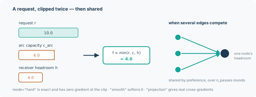
Rule-based allocation of water between stores. Nodes are stores (reservoirs, treatment works, demand points) with a storage ceiling; edges are arcs with a capacity. Each arc carries the flow that is requested of it, clipped to the arc's capacity and to the free storage at the receiving node, and storage is conserved exactly at every node. Requests and flows are in m³/s, storage in m³. In noodl physics this is implemented by AllocatedFlowLayer, and it is the framework's fourth flow-determination mode.

Every other application on this site determines a flow from physics: a potential difference, a closure, or continuity. This one does not. Each edge carries a requested flow, typically emitted by an upstream process rather than a pressure difference, and the layer clips it against two independent bounds — the edge's own capacity, and the receiving node's remaining storage headroom. There is no potential variable anywhere in the calculation.

\[ f = \min\left(r,\; c_{\text{arc}},\; h_{\text{receiver}}\right) \]

This is push/pull semantics. An edge pushes a request at its target; the target accepts up to its own headroom; the difference is left unmet at the source. Conservation is exact by construction.

It is a genuinely different mode, not a variant of the Kirchhoff layer. Water-resources networks — abstraction licences, reservoir operating rules, treatment-works throughput — are governed by rules, and the rule is the physics.

from noodl.layers.allocation import AllocatedFlowLayer

Every type this application offers — what it does and how to call it — is listed in its catalogue. It is set up and run like every other model; see Using noodl.

A worked example

import torch
from noodl.layers.allocation import AllocatedFlowLayer
from noodl.topology import Network

F64 = torch.float64

net = Network()
for n in ("A", "B", "C"):
    net.add_node(n)
net.add_edge("A", "B", kind="link")
net.add_edge("B", "C", kind="link")

layer = AllocatedFlowLayer(
    net, "cap", "link",
    s_max=torch.full((net.n,), 100.0, dtype=F64),
    c_arc=torch.full((2,), 10.0, dtype=F64),
)

s0 = torch.zeros(net.n, dtype=F64)
drivers = {"cap.requests": torch.tensor([2.0, 2.0], dtype=F64)}
s1, f = layer.step(s0, drivers, dt=1.0)

# f  == [2.0, 2.0]   — both requests pass through
# s1 == [-2.0, 0.0, 2.0]
#   A is only a source and loses 2; B gains 2 and loses 2; C gains 2.

(From tests/layers/test_allocation.py.) Two adjacent tests show the clip branches: with c_arc = 1.5, requests of [5.0, 5.0] give f = [1.5, 1.5]; with node C already full, requests of [2.0, 2.0] give f = [2.0, 0.0].

Note that s1[0] is negative. step bounds storage from above only — a source node may be drawn below zero, which is a modelling choice belonging upstream of this layer.

From a WSIMOD topology

noodl.apps.wsimod.build_model(topology) builds the layer and a Model from a WSIMOD-style topology ({"nodes": [{"name"}], "arcs": [{"name", "source", "target", "capacity"}]}, or a JSON file of it) and returns (model, state, drivers) like the other applications. Requests and storage are then given by arc and node name:

from noodl.apps import wsimod

model, state, drivers = wsimod.build_model("quickstart_topology.json")
state = wsimod.initial_state(model, values={"wsimod": {"my_groundwater": 5.0}})
drivers = wsimod.initial_drivers(model, values={"wsimod.requests": {"baseflow": 0.3}})
state = model.step(state, drivers, dt=86400.0)

See Using noodl.

The API

The allocation rules (push/pull requests, the per-arc capacity clip and the receiver's headroom check) follow those of WSIMOD, Imperial College's Water Systems Integrated Modelling framework. Sharing between arcs competing for one node's headroom does not: WSIMOD serves such requests first come, first served, and this layer shares preference-proportionally (see where the layer differs from WSIMOD).

AllocatedFlowLayer has exactly two public methods.

AllocatedFlowLayer(
    net, name, kind, *,
    s_max,            # per-node storage ceiling, trailing shape (net.n,); inf for unbounded
    c_arc,            # per-edge arc capacity, in this kind's edge order
    preference=None,  # per-edge sharing weight, strictly positive; None means all ones
    mode="hard",      # 'hard' | 'smooth' | 'projection'
    tau=None,         # temperature; required for mode='smooth'
    n_passes=5,       # fixed sharing rounds
)

s_new, f = layer.step(s, drivers, dt, *, diagnostics=None)

step reads f"{name}.requests" from drivers (per edge, m³/s) and returns the new per-node storage and the realised per-edge flow. diagnostics, when given, is filled with "overflow" in m³/s per node — reported, never fed back.

dt is load-bearing. Headroom is converted to a rate, \((s_{\max} - s)/\Delta t\), so the clip bounds the actual storage increase at any timestep, not only at \(\Delta t = 1\). This is regression-tested at \(\Delta t = 2\) and \(\Delta t = 86400\).

preference must be strictly positive. Projection mode divides by it live, and a non-positive weight would give a clean forward value with a silent NaN gradient.

In a Model, an allocation layer steps between the potential solves and the transport steps, so a transport layer reading "<layer>.q" sees a freshly written flow whichever kind of layer wrote it. A model owning one refuses a steady pass and refuses residuals() — a clip-and-allocate rule is inherently discrete-time and has no steady meaning to report.

The three modes

They compute the same thing. They differ in what the gradient does, and that is the entire reason there is more than one.

"hard" — exact, and zero-gradient at the clip

Plain minimum and clamp. Bit-identical to the bare clip formula, untouched by the existence of the other modes. This is what WSIMOD parity is measured against.

Differentiable almost everywhere — but at and near a capacity or headroom crossing the gradient through the discrete branch choice is exactly zero. A node moving from "headroom covers demand" to "oversubscribed" carries no gradient signal across that boundary.

Use it for forward simulation, and for training that never crosses a binding constraint.

"smooth" — a live gradient across the boundary

minimum becomes a softmin, \(-\tau \log\sum e^{-a/\tau}\); clamp becomes a softplus; and the branch selection itself is smoothed by a sigmoid-weighted blend of two whole branches, not just the arithmetic inside each. That last part is the point: smoothing only the arithmetic would leave the discrete choice, and its zero gradient, in place.

The cost is an \(O(\tau)\) forward bias. The measured 1.79e-3 discrepancy in the parity table below is not capacity-smoothing residue — every arc in that fixture is unbounded, so the softmin is exact to float64. It is the softplus-at-zero bias, \(\tau \ln 2 \approx 6.9\times10^{-4}\) at \(\tau = 10^{-3}\), at kink sites many requests sit exactly on, compounding through recurrent storage.

Use it when you need a gradient across a capacity boundary but only care about self sensitivity.

"projection" — real cross-gradients between competing edges

Smooth mode's proportional-share formula is \(h_{\text{free}} \cdot \text{pref}_i / \sum_k \text{pref}_k\). That depends only on the preference weights and the total headroom — never on any individual competitor's request. So \(\partial f_i / \partial r_j = 0\) for a competing edge \(j\), provably and not approximately. It is confirmed empirically too: byte-identical zero cross-terms across 200 random trials. That formula cannot deliver a genuine cross-gradient — gradients flowing through which arc absorbs a constraint — however it is wrapped, which is why projection mode routes the sharing site through a real coupled QP instead: minimise \(\sum_i \text{pref}_i (f_i - r_i)^2\) subject to \(0 \le f_i \le \text{avail}_i\) per edge and \(\sum_i f_i \le h_{\text{free}}\) jointly. Its KKT stationarity reduces to

\[ f_i = \operatorname{clamp}\!\left(r_i - \frac{\lambda}{\text{pref}_i},\ 0,\ \text{avail}_i\right) \]

for one scalar \(\lambda\) shared by every edge competing at that node — and \(\lambda\) is the unique root of a monotone scalar equation, which is exactly solve_monotone's contract.

That shared multiplier is what produces a genuine cross-gradient:

\[ \frac{\partial f_i}{\partial r_j} = -\frac{1/\text{pref}_i}{\sum_k 1/\text{pref}_k} \]

On a symmetric-preference diamond this gives \(\partial f_{BD} / \partial r_{CD} = -0.5\), which was hand-derived and is checked for both sign and magnitude. The general formula was separately hand-verified against asymmetric fixtures (pref=[1,3] → \(-0.25\); pref=[1,2,5]) to four decimal places. That confirms the mechanism generalises — not that \(-0.5\) itself does.

A full Newton treatment of the QP was considered and rejected: it would need a Fischer-Burmeister-smoothed complementarity condition, which is a harder-to-verify reimplementation of what smooth mode already does, for no accuracy benefit.

Proportional sharing and n_passes

Sharing happens only at a node that is the target of more than one edge. A node with a single in-edge is never touched, however many out-edges lie downstream: this layer never caps an edge to match a bottleneck further along the graph. That matches WSIMOD for storing nodes (Storage, Waste), whose accept decision is a check against their own headroom. It does not match a WSIMOD pass-through Node, which accepts only what it can forward in the same step (see where the layer differs from WSIMOD).

Each of the n_passes rounds computes a tentative flow, finds the nodes whose summed demand exceeds their free headroom, and on those nodes replaces the tentative flow with a preference-weighted share — with preference renormalised over the edges still actively competing, so an edge that already got everything it asked for does not soak up a share it no longer wants.

That renormalisation is what n_passes is for. Three edges into one sink with headroom 3.0, equal preference, requests [0.5, 10.0, 10.0]:

Passes	Realised	Total
1	[0.5, 1.0, 1.0]	2.5 — under-uses the headroom by 0.5
2	[0.5, 1.25, 1.25]	3.0 — X's freed weight redistributes
5	[0.5, 1.25, 1.25]	3.0 — already converged at pass 2

remaining only shrinks and f only grows round over round, so more passes move a share closer to the true max-min-fair split and never past it. The default of 5 matches WSIMOD's own constants.MAXITER; WSIMOD uses a while loop with early exit, and noodl physics uses a fixed count for batched differentiability — each round is strictly non-expansive, so a fixed cap is a safe over-approximation rather than a different algorithm.

Storage, requests, capacities and preferences may each carry their own leading batch dimensions: step broadcasts them to one common batch shape, so a batch of requests runs from a single unbatched initial storage (or a batched capacity from unbatched requests).

Verification

Against WSIMOD 0.8.1 (Dobson, Liu and Mijic), pinned exactly rather than with >=, because the committed fixtures freeze one specific WSIMOD run and a newer release could silently change the demos' forcing or node parameters.

The harness monkeypatches Arc.send_push_request / send_pull_request to capture every per-arc requested/realised pair while WSIMOD runs its own quickstart_demo and oxford_demo. The committed fixtures mean the parity tests run without WSIMOD installed.

Check	Tolerance	Measured
Hard clip vs WSIMOD's realised flows, quickstart_demo, all 1,456 steps	1e-9 abs	1.11e-16
Same, oxford_demo, 20 of 21 arcs	1e-6 abs	1.86e-9
"smooth" at \(\tau=10^{-3}\) vs the hard clip's own output on quickstart_demo	3e-3 abs	1.79e-3
"projection" vs the hard clip's own output on quickstart_demo	1e-9 abs	9.10e-13
Conservation, both demos, all three modes	exact	holds, no reference needed
gradcheck through smooth and projection on the diamond	analytic	holds
n_passes=5 vs a hand-converged reference	exact	holds
Scripted WSIMOD networks with binding arcs and tanks (6 cases, dt = 86400 s): realised volumes and storage	1e-12 × case scale	≤ 4.4e-16
quickstart_tight (three arc capacities lowered), all 6 arcs, 1,456 steps	1e-12 × 0.113	1.04e-16

Binding capacities and headroom

The two shipped demos never bind: all but one of their 27 arcs sit at WSIMOD's UNBOUNDED_CAPACITY of 1e15, the one finite arc (abstraction_to_farmoor, 50000) never sees a request above about 30,934, and the replay sets \(s_{\max} = \infty\). On their own they check only the identity path, \(\min(x, c) = x\).

tests/verification/test_wsimod_capacity.py covers the binding branches against WSIMOD's own numbers. It runs small networks built from WSIMOD's own Arc, Node, Storage and Waste classes, driven by WSIMOD's push_distributed and pull_distributed, and checks from WSIMOD's output that each targeted bound really cut a request before it compares:

• a push clipped by arc capacity, with one or several requests in a timestep;
• a push and a pull on the same arc in one timestep, sharing its capacity;
• a tank whose headroom and inflow-arc capacity bind in turn as its storage evolves;
• WSIMOD's preference-weighted push_distributed and pull_distributed, where a round's request exceeds an arc's capacity and WSIMOD's own clip cuts it.

It also replays quickstart_tight, which is quickstart_demo with runoff, baseflow and percolation lowered to 0.03, 0.04 and 0.08. WSIMOD cuts baseflow to its capacity on 1,085 days. runoff and percolation run at capacity on 866 and 552 days, but WSIMOD's Land node sizes those requests from the arc's own check, so there request = capacity.

WSIMOD clips each request against capacity - flow_in, and flow_in accumulates every push and pull already realised on the arc in that timestep. The split between requests therefore depends on their order, but the timestep total is \(\min(\sum_k r_k, c)\) in any order, and that total is what one layer step computes from the summed request.

Where the layer differs from WSIMOD

These differences are tested, not tolerated:

• Several arcs competing for one node's headroom. WSIMOD serves them in call order. The layer shares by preference and ignores order. Two 10-unit pushes into 12 units of headroom give [10, 2] or [2, 10] in WSIMOD, depending on which is called first, and [6, 6] in the layer. The total and the storage agree. WSIMOD's own proportional sharing happens earlier, when a sender or puller sizes its requests, so it is already in the requests the layer replays.
• Same-step outflow. The layer uses the headroom at the start of the step. WSIMOD frees headroom for an inflow if an outflow is called first.
• Bottlenecks behind a pass-through node. A WSIMOD Node forwards each push immediately and hands back what it cannot forward, so a tight arc downstream also limits the arcs feeding it. The layer is receiver-local. With quickstart_demo's catchment_outflow lowered to 0.1, that arc replays exactly, but baseflow and storm_outflow differ by up to 0.24 and 0.04.
• Node-level limits. These are source availability on a pull, and throughput caps such as oxford_demo's WWTW node. That is why sewer_to_wwtw is left out of the oxford_demo comparison (20 of 21 arcs compared): it mismatches on 185 of 1,456 steps, although its own capacity is 1e15.
• Not compared at all. QueueArc and DecayArc travel time and decay, force=True pushes, and pollutants. The layer does not model any of them.

Throughput

Run	Measured
oxford_demo topology (21 arcs, 18 nodes), hard clip, 1,456 steps	batch 1: 1.004 s; batch 10: 1.338 s; batch 100: 1.439 s

WSIMOD's own single-instance run takes about 4 s, but that is not a fair batched-against-unbatched comparison and no budget is set on it. The benchmark also carries its own caveat: with \(s_{\max} = \infty\) everywhere, no node is ever oversubscribed, the sharing branch never runs, and every pass after the first is a no-op. It measures the cheapest path only.

Out of scope

• The WSIMOD Node wrapper — embedding a noodl physics Model as a live WSIMOD node via push_set/pull_set — is deferred.
• The other nine WSIMOD pollutants. The layer is species-count-agnostic, so this is a matter of widening a transport layer's species list and the fixture capture, not a change here.
• Species and quality transport riding on an allocation layer is not wired up.
• Time-varying arc capacities and storage bounds — construction-time buffers only, since WSIMOD's own capacities are static within a run.

Install

Nothing beyond the base dependencies. wsimod==0.8.1 is needed only to regenerate the fixtures; the parity tests themselves read the committed ones.