Applications

noodl physics is one solver. The applications below are physical systems modelled with it, each a thin layer of domain physics (its constitutive laws, drives and closures) over the shared core. Any of them can be built directly in Python, as each page shows, or, where a reader exists, read from a model file; see File formats. Every application is initialised the same way, with initial_state(model, values=...) and initial_drivers(model, values=...) by name; see Using noodl. The electrical application has no initial_drivers: its build_model returns every driver, and initial_state(model, drivers) solves the consistent initial point of the circuit.

Application	Physical system	Flow determination	Entry point
Building physics	Multi-zone airflow, heat, contaminants	Kirchhoff: Newton on zone pressure	build_model
Street air quality	Urban air quality, canyon exchange, routing	Closure: flows computed from the wind aloft	build_model, StreetNetwork
Sewers	Gravity hydraulics, headspace air, sulfide	Continuity on a tree for the water (kinematic wave), or Kirchhoff solve on head (dynamic wave); Kirchhoff solve for the headspace air	build_model
Water distribution	Pressurised mains, pumps, tanks, demand	Kirchhoff: Newton on hydraulic head	build_model
Flow allocation	Requested flows clipped to arc capacity and free storage at the receiving node	Clip and allocate	AllocatedFlowLayer, wsimod.build_model
Electrical circuits	Lumped circuits: DC, transient and AC	Kirchhoff: Modified Nodal Analysis on node voltage	build_model, Circuit
Coupling	Two models meeting at a shared boundary	Two models exchanging values, iterated to a fixed point	union

Why these seven

They are not a feature list. They are the argument that the factorisation works.

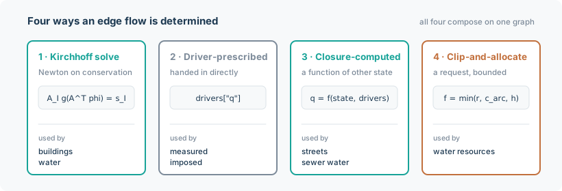
Each uses a different one of the four flow-determination modes, and between them they cover all four:

• The building physics and water applications solve for a potential — pressure in pascals, hydraulic head in metres. Newton on a nodal conservation residual.
• The street air quality application has no potential at all. The along-canyon velocity is a closed-form function of the wind aloft, so a closure computes every flow directly.
• The sewer application's kinematic-wave water side exploits the fact that a tree has an empty cycle space: continuity alone fixes every discharge, in closed form, with no solve. Its dynamic-wave water side is a Kirchhoff layer on head, iterated to SWMM's fixed point, and admits loops and backwater. Its headspace air side, on the same graph, is a full Newton Kirchhoff solve.
• The flow allocation application has no potential and no continuity solve — a request, clipped against capacity and headroom.
• The electrical circuits application solves for a potential, the node voltage, with the currents of ideal sources, inductors and transformers as extra unknowns: Modified Nodal Analysis, the full form of the nodal solve the building and water applications use.

And they share machinery in ways that would be coincidence if the abstraction were wrong. The sewer's headspace air layer drives its Newton solve with the same Stack buoyancy term the building application uses for room air. The water application's Darcy-Weisbach pipes can be the framework's own Duct element in volumetric form (friction="colebrook"), though by default they follow EPANET's own composite friction law. The sewer and water .inp readers share one tokenizer. The solve_monotone root-finder that inverts Manning's equation for sewer depth also solves the per-node QP inside the allocation layer's projection mode.

Verification

Each application page ends with a Verification section: code-to-code comparisons against established reference models that solve the same equations (CONTAM and ContamX and the Modelica Buildings Library for building physics, MUNICH for street air quality, SWMM through pyswmm for sewers, EPANET 2.2 through WNTR for water distribution, WSIMOD for flow allocation, the Modelica Standard Library and pandapower for electrical circuits), plus checks against analytical solutions, conservation identities and finite-difference gradients.

A comparison of this kind runs noodl physics and a reference model on the same input and compares the outputs at a stated tolerance. It shows that noodl physics solves the same model as the reference; it is not evidence that the model describes reality. Where the reference model has not been run, as for MUNICH on this release, the check is instead against the formulas and published results the reference documents, and the application page says so. Validation, comparison against measurements, is not claimed by any application yet.

Each page states its comparisons with an explicit tolerance and the value actually measured. The pages are equally explicit about what a comparison does not show, and those caveats are sometimes the most important thing on the page:

• The flow allocation page explains that WSIMOD's shipped demos never exercise a binding clip, how scripted WSIMOD cases cover those branches instead, and where the layer's semantics differ from WSIMOD's: sharing one node's headroom, and bottlenecks behind a pass-through node.
• The street air quality page records that the published MUNICH idealised case cannot be reproduced absolutely, because its geometry was never published, and states the size of the remaining difference.
• The sewer page marks each coefficient as verified, calibrated, or unverified, naming the source.

Where a reference model and noodl physics disagree, the pages say which is more likely to be right and why. Several of the remaining discrepancies are the reference's approximation — SWMM's 51-point circular-geometry lookup table, EPANET's float32 binary output — not noodl physics'.

Starting a new application

The seven are also a template. A new application is:

1. A network builder — domain dataclasses plus a function that turns them into a Network with the right edge kinds and attributes.
2. Constitutive laws and drives for whatever laws are not already in the core.
3. Closures for anything that is a function of solved state.
4. A file reader, if your field has a standard exchange format.
5. A build_*_model function returning (model, state, drivers), and a *_steady helper if reactions mean Model.steady is not enough.

Every application follows exactly that shape, which makes them readable as worked examples.