Networks

noodl.topology.Network is the typed multigraph every model is built on. It owns the graph and every operator derived from it — incidence, gradient, cycle basis, spanning forest, boundary and interior selectors — and caches them, so building a layer costs the derivation once.

Building one

import torch
from noodl.topology import Network

net = Network(dtype=torch.float64)
net.add_node("ambient")
net.add_node("room", volume=60.0, z_ref=0.0)
net.add_edge("room", "ambient", kind="airpath", area=0.05, Cd=0.6)

Nodes and edges carry arbitrary attributes. Those attributes are how an application passes geometry to its elements: orifice_law_from_edges reads Cd and area off every edge of a kind, and thermal_layer reads volume off every node. Attributes are retrieved in bulk and as tensors, never one at a time:

volumes = net.node_attr("volume", default=0.0)     # (n,) tensor, full node order
areas = net.edge_attr("area", kind="airpath")      # (b_kind,) tensor, kind order

Edge kinds

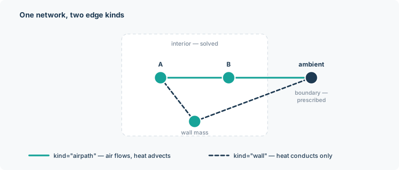
Every edge has a kind, and every operator takes an optional kind argument that restricts it to those edges. This is the mechanism that lets one network hold several physical systems:

net.add_edge("room", "ambient", kind="airpath")   # air can flow
net.add_edge("room", "wall", kind="wall")          # heat conducts, air does not

A Kirchhoff layer solving on "airpath" never sees the wall edges. A thermal layer advecting on "airpath" and conducting on "wall" sees both, in separate blocks. The sewer application uses this to put water, headspace air and two quality layers on one graph; the street application uses it to separate route, vent and exchange edges.

net.edge_kinds()            # ['airpath', 'wall']
net.edge_index("airpath")   # positions of that kind's edges in full edge order

The operators

These are the graph-theoretic core. All are cached, all take a kind, and all move with .to(device, dtype).

Method	Returns
incidence(kind=None)	\(A\), the \(n \times b\) signed node-edge incidence matrix.
gradient(kind=None)	\(A^\top\), mapping nodal potentials to potential differences along edges.
difference(kind=None)	The same difference operator in the form layers consume.
cycle_basis(kind=None)	A basis for the cycle space: \(n_{\text{cycles}} = b - n + n_{\text{islands}}\).
spanning_forest(kind=None)	Tree and chord edge indices — a tree has an empty cycle space, which is what makes the sewer's flow solve closed-form.
endpoints(kind=None)	(source_idx, target_idx) per edge, for matvec-free assembly.
accumulate(w, kind=None)	Scatter-adds an edge quantity to its endpoints with sign — nodal balance, without ever forming \(A\).
source_selector / target_selector	Selection matrices for the two endpoints.
upwind(q, kind=None) / downwind(q, kind=None)	Sign-aware indexing: which endpoint is upstream given the flow direction. This is what makes advection work on a graph whose edge orientations are arbitrary.

The accumulate / endpoints pair matters more than it looks. Layers assemble their operators through them rather than through a dense \(A\), which is why a large network never materialises an \(n \times b\) matrix and why the linear operators are matvec-free. See Solvers.

Boundary and interior

A node is boundary if its potential (or state) is prescribed rather than solved. Everything else is interior. You name the boundary when you build a layer, and the network turns that into index tensors:

interior = net.interior_index(["ambient"])   # solved nodes
boundary = net.boundary_index(["ambient"])   # prescribed nodes

Boundary names may be aliases of nodes merged by components; net.canonical(names) returns the node names they refer to, and both index methods raise ValueError when two of the names are the same node.

n, b, n_islands and n_cycles report the sizes. island_labels(kind) and n_islands_of(kind) do the same restricted to a kind, which is how a layer discovers whether its subgraph is connected — a disconnected potential problem needs one grounded node per island, and the solver will tell you so rather than silently returning a singular result. See Solvers.

An island is a part of the network with no path to the rest; a building whose airflow network has two islands has two air systems that never exchange air.

Ambient

Most physical networks want a single node representing "outside". with_ambient adds one and returns the network for chaining:

net = Network(dtype=torch.float64).with_ambient("ambient")

Tellegen's theorem

This structure guarantees an identity worth naming directly. For any nodal potentials \(p\) and any flows \(q\) satisfying nodal conservation,

\[ \sum_{\text{edges}} (A^{\top} p)_e \, q_e = 0 . \]

Potential differences live in the cut space, conservative flows live in the cycle space, and the two are orthogonal complements. The branch power sum is therefore zero regardless of what the elements are — it is a property of the graph, not of the physics.

residual = net.power_residual(p, q)   # zero to machine precision for a conservative q

This is not decoration. It is a free, physics-independent check on any solve, and the applications use it as one: the sewer application's headspace air layer pins its own power residual below \(10^{-10}\,\)W (measured \(6.1\times10^{-12}\)), and the street application checks that every kilogram emitted crosses the atmosphere boundary exactly. A model that violates Tellegen has a bug in its conservation, and the identity catches it without a reference solution. The theory page develops this properly.

Devices and dtype

net = net.to(device="cuda", dtype=torch.float64)

Every cached operator moves with it. The default dtype is float32; the applications all override to float64, and you should too for anything involving a Newton solve with a tight tolerance.

Cycles

noodl.cycles works in the cycle space directly, which is what you need when flows are measured rather than solved:

Function	Purpose
branch_flows(net, amplitudes, kind)	Turns cycle amplitudes into branch flows. Any such flow conserves at every node by construction.
particular_flow(...)	A particular conservative flow matching prescribed nodal sources. On a tree this is the whole answer, which is how the sewer application solves its hydraulics without a Newton solve at all.
project_measured(...)	Projects measured flows onto the conservative subspace — the least-squares correction that makes an inconsistent set of measurements satisfy continuity.
assert_forward_oriented(net, kind)	Checks every edge of a kind points the way the physics assumes.

The coupling application's third inverse example uses project_measured to recover all four branch flows of a network from one measured path, exactly (rtol \(10^{-10}\)).