7. Fractal geometries#
In the previous chapter we encountered a paradox. The Lorenz equations are dissipative, so that every volume of initial conditions in phase space shrinks to zero as \(t\rightarrow\infty\). At the same time, the trajectories cannot settle onto a fixed point or a limit cycle, but are confined to the strange attractor on which they display a sensitive dependence on initial conditions. The attractor can therefore have no volume, yet it cannot be a simple surface either, as this would be incompatible with the chaotic dynamics. We resolved this paradox by claiming that the geometry of the attractor is fractal, with a dimension that is not an integer but lies somewhere between two and three.
The purpose of this chapter is to put this notion of a non-integer dimension on a firmer footing. We will first introduce fractals through a number of classical geometric constructions, for which the dimension can be obtained analytically from the self-similarity of the object. We then turn to the more general box-counting dimension and the correlation dimension, both of which can be determined numerically for an arbitrary set of points, such as a measured strange attractor. Finally, we consider objects for which a single dimension is not sufficient, the multifractals, and characterize these by a whole spectrum of generalized dimensions \(D_q\).
7.1. Self-similar fractals#
A geometrical object is called self-similar when it is built up out of smaller copies of itself. The prototypical example is the von Koch curve, constructed by the recursive procedure sketched in Figure 7.1. One starts with a straight line segment of unit length (the initiator). This segment is replaced by four segments of length \(1/3\), the middle two forming a triangular bump (the generator). The same operation is then applied to each of the four new segments, and so on ad infinitum. The limiting curve is continuous everywhere but differentiable nowhere, and has an infinite length.
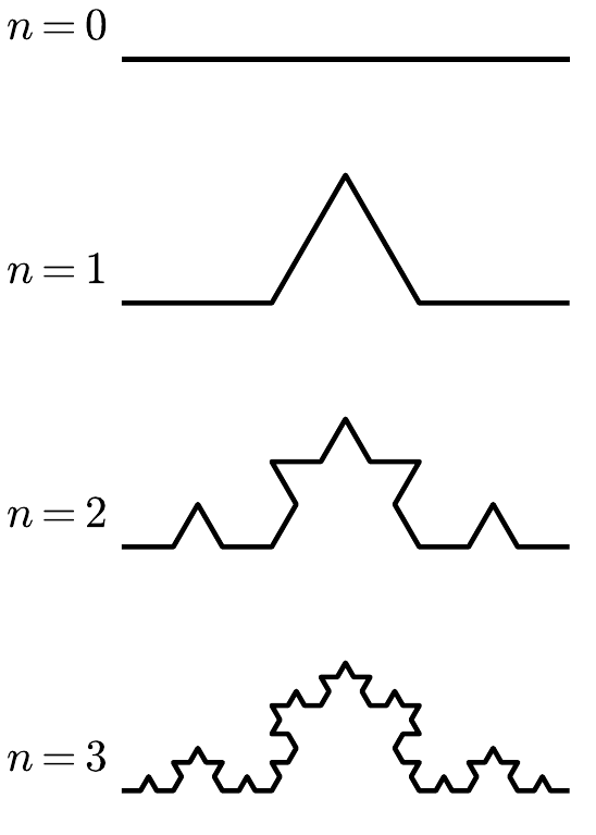
Figure 7.1 Construction of the von Koch curve. At each step every segment is replaced by four segments of one third of its length.#
Maple
The recursion is short to code. Representing the points of the curve as complex numbers, the generator replaces each segment by four, the extra vertex being the first third rotated by \(\pi/3\) to raise the bump.
restart: with(plots):
gen := proc(p, q) local d:                   # Koch generator for one segment
  d := (q - p)/3:
  p, p+d, p + d + d*exp(I*Pi/3), p + 2*d:     # its four leading vertices
end proc:
pts := [0, 1]:                               # unit segment (points as complex)
for k to 4 do                                # replace every segment, four times
  pts := [seq(gen(pts[i], pts[i+1]), i=1..nops(pts)-1), pts[-1]]:
end do:
plot([seq([Re(z), Im(z)], z in pts)], scaling=constrained);
To assign a dimension to such an object, we recall how the ordinary dimension of a simple geometrical shape can be characterized. Consider covering the shape with smaller copies of itself, each scaled down by a factor \(s<1\). A line segment of unit length is covered by \(N=1/s\) copies of length \(s\); a square by \(N=(1/s)^2\) copies of side \(s\); a cube by \(N=(1/s)^3\) copies of side \(s\). In each case the number of copies scales as
where \(D\) is the (integer) dimension of the object. Taking the logarithm of (7.1) and solving for \(D\) suggests the following definition of the similarity dimension of a self-similar object:
where \(N\) is the number of copies and \(s\) the scaling factor of each copy. Crucially, nothing in (7.2) forces \(D\) to be an integer.
For the von Koch curve, each segment is replaced by \(N=4\) copies scaled down by \(s=1/3\), so that
The dimension is larger than one, reflecting the fact that the curve is so convoluted that it starts to fill the plane, but it is smaller than two because it does not fill any area. It is precisely this kind of non-integer dimension that we anticipated for the strange attractor. By altering the generator – for instance replacing the middle bump by four equal segments set at a different angle – one can construct self-similar curves of any dimension between one and two, so that the dimension is a design parameter rather than a fixed number.
Two further classical constructions will accompany us throughout this chapter. The Cantor set (Figure 7.2) is obtained by repeatedly removing the middle third of a line segment: the unit interval is replaced by its two outer thirds, each of these by their outer thirds, and so on. At each stage the set consists of \(N=2\) copies scaled by \(s=1/3\), so that
The Cantor set is an example of a dust: its dimension lies between zero (a point) and one (a line). Although it contains uncountably many points, it has zero total length.
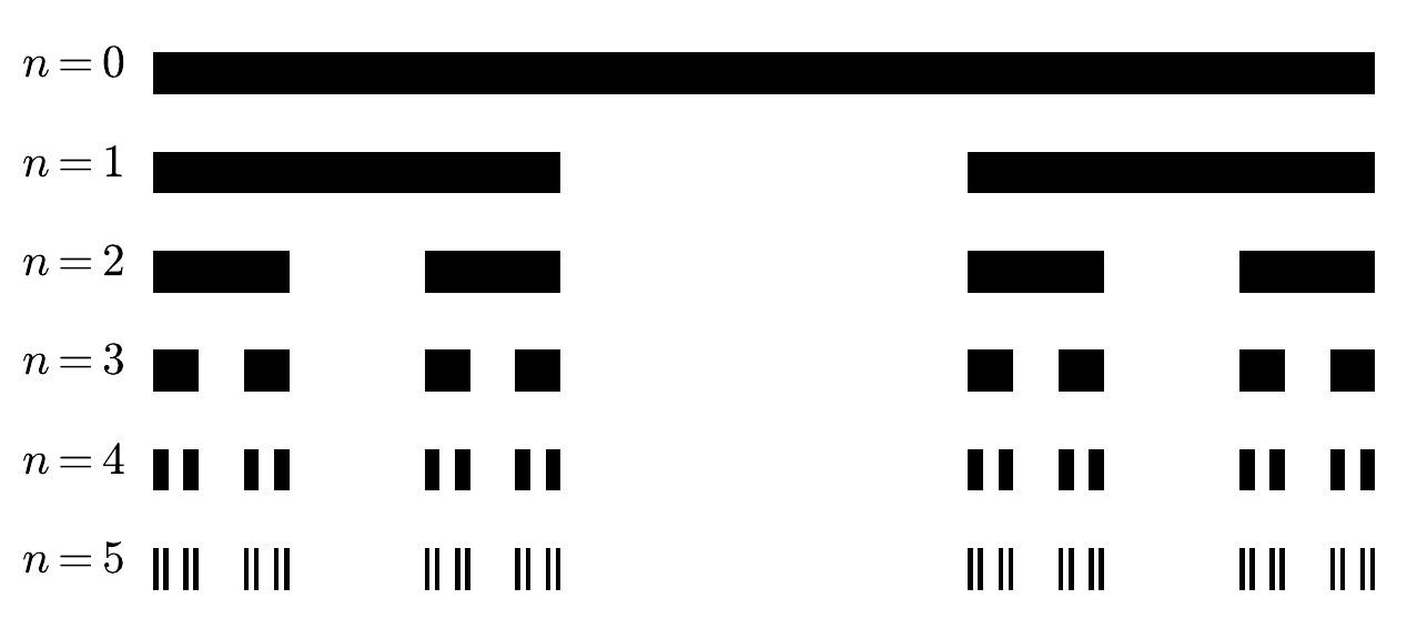
Figure 7.2 The middle-third Cantor set. At each stage the central third of every segment is removed.#
The two-dimensional analogue is the Sierpinski gasket (Figure 7.3). An equilateral triangle is divided by the midpoints of its sides into four congruent sub-triangles, and the central, inverted one is removed. Each of the three remaining triangles is treated in the same manner recursively. Here \(N=3\) and \(s=1/2\), so that
As expected the dimension lies between one and two: the gasket is pierced by holes on every scale, yet its remaining filaments still branch too densely for it to be a mere curve.
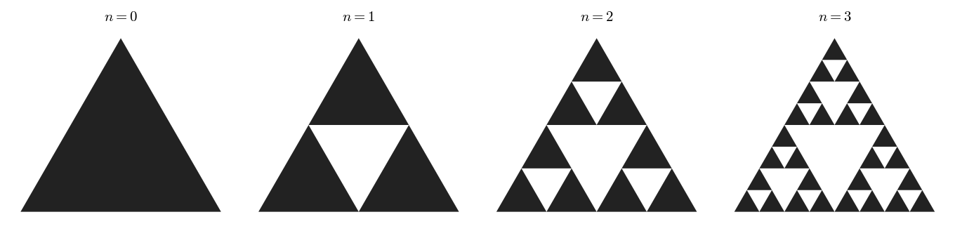
Figure 7.3 The first iterations of the Sierpinski gasket.#
Example
Self-similar reasoning can also be applied to areas and perimeters simultaneously. The Koch island is generated by applying the von Koch construction to each of the three sides of an equilateral triangle (Figure 7.4). The perimeter is a von Koch curve, and therefore has fractal dimension \(D=\log 4/\log 3\). If the initial perimeter has length \(P_0=3\), then after \(n\) steps each segment has been replaced by four segments of one third the length, so that the perimeter
diverges. The enclosed area, on the other hand, remains finite. At each step a new triangular bump is added to every segment; summing the resulting geometric series shows that \(A_n\) converges to \(A_\infty = \tfrac{8}{5}A_0\). Consequently the hydraulic diameter \(D_n = 4A_n/P_n \rightarrow 0\): the island encloses a finite area behind an infinitely long, infinitely wrinkled coastline. This is the sense in which Mandelbrot [1967] famously asked how long the coastline of Britain really is.
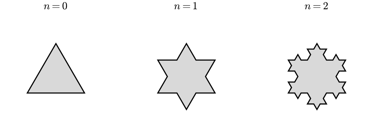
Figure 7.4 Construction of the Koch island.#
7.2. The box-counting dimension#
The similarity dimension (7.2) is only defined for objects that are exactly self-similar. A strange attractor obtained from a numerical simulation or an experiment is not built by an explicit recursive rule, and we need a definition of dimension that can be applied to any set of points. The box-counting dimension provides exactly this, and is in this sense the more fundamental of the two: it is defined for any bounded set and is what one actually measures from data, while the similarity dimension is recovered as the special case in which exact self-similarity lets the boxes be counted by hand.
The idea is to cover the object with a grid of boxes of size \(\varepsilon\) and to count the number \(N(\varepsilon)\) of boxes that contain at least one point of the set. For a smooth curve of length \(\ell\), the number of boxes needed scales as \(N(\varepsilon)\sim \ell/\varepsilon = \ell\, \varepsilon^{-1}\); for a smooth surface of area \(\mathcal{A}\) it scales as \(N(\varepsilon)\sim \mathcal{A}\, \varepsilon^{-2}\). In general one expects
which motivates the definition of the box-counting dimension
For the exactly self-similar objects of the previous section the box-counting dimension coincides with the similarity dimension: choosing \(\varepsilon = s^{k}\) at the \(k\)-th generation, one needs exactly \(N=N_{\text{copies}}^{k}\) boxes, and (7.7) reproduces (7.2). The subscript \(0\) in \(D_0\) anticipates the family of generalized dimensions introduced in section 7.4; the box-counting dimension is the member \(q=0\) of that family.
In practice one cannot take the limit \(\varepsilon\rightarrow 0\), both because a data set contains a finite number of points and because a numerically generated fractal is only self-similar down to some smallest scale. Instead one evaluates \(N(\varepsilon)\) for a range of box sizes and estimates \(D_0\) from the slope of \(\log N(\varepsilon)\) versus \(\log(1/\varepsilon)\). According to (7.6), a plot of \(\log N\) against \(\log\varepsilon\) should be a straight line of slope \(-D_0\) over the range of scales where the object is fractal.
Example
Box-counting the von Koch curve makes the yardstick idea precise. Covering the curve with boxes of size \(\varepsilon = 3^{-k}\), each of the \(4^{k}\) segments of the \(k\)-th generation lands in a single box, so that \(N(\varepsilon) = 4^{k}\) and
exactly the similarity dimension (7.3). Equivalently, measuring the curve with a ruler of length \(\varepsilon\) returns an apparent length \(L(\varepsilon) = N(\varepsilon)\,\varepsilon \propto \varepsilon^{\,1-D_0}\), which diverges as \(\varepsilon\rightarrow 0\): the finer the yardstick, the longer the coastline. Running the box-counting program below on a set of points sampled along the curve recovers the same slope numerically.
The maple program below implements the box-counting procedure for a set of \(N\) points \((x_n,y_n)\) in the plane, as would be obtained from the return plot of an experimental time series (here the dripping-faucet data of chapter 3). The box size is halved repeatedly by increasing the integer exponent \(p\), so that \(\varepsilon = (x_{\max}-x_{\min})/2^{p}\).
Maple
restart; with(plots): with(stats):
dat := readdata("D1.drip", [float]):
N   := nops(dat)-1;
x   := [seq(dat[n],   n=1..N)]:
y   := [seq(dat[n+1], n=1..N)]:
xmin := min(x[]): xmax := max(x[]):
ymin := min(y[]): ymax := max(y[]):
loli := NULL:
pmin := 1: pmax := 7: dp := 0.2:
for p from pmin to pmax by dp do
  delta := (xmax-xmin)/2^p;              # current box size
  ni := trunc((xmax-xmin)/delta)+1;
  nj := trunc((ymax-ymin)/delta)+1;
  nr := Matrix(ni, nj, 0);               # occupancy grid
  for n from 1 to N do                   # mark every occupied box
    i := trunc((x[n]-xmin)/delta)+1;
    j := trunc((y[n]-ymin)/delta)+1;
    nr[i,j] := 1;
  end do:
  boxes := add(add(nr[i,j], j=1..nj), i=1..ni);
  loli  := loli, [log(delta), log(boxes)];
end do:
xli := [seq(loli[k][1], k=1..nops([loli]))]:
yli := [seq(loli[k][2], k=1..nops([loli]))]:
eq  := fit[leastsquare[[x,y], y=a*x+b]]([xli, yli]);   # slope = -D0
The final least-squares fit returns a line \(y = a\,x + b\) with \(x=\log\delta\) and \(y=\log(\text{boxes})\). By (7.6) the box-counting dimension is \(D_0 = -a\), i.e. minus the slope. Applying this procedure to the Sierpinski gasket of Figure 7.3 recovers the analytical value \(\log 3/\log 2\), provided that enough points are used. This last caveat is important: the box-counting method only works over the range of scales that is adequately sampled by the data. When the number of points \(N\) is too small, the finest boxes each contain at most one point, \(N(\varepsilon)\) saturates at \(N\), and the estimated slope flattens out. As a result, too few data points always lead to an underestimate of the dimension at small \(\varepsilon\) (Figure 7.5). A complete, self-contained version of this pipeline – generating a self-similar point set, counting occupied boxes over a range of sizes, and extracting the slope by a least-squares fit – is worked through in the cookbook.
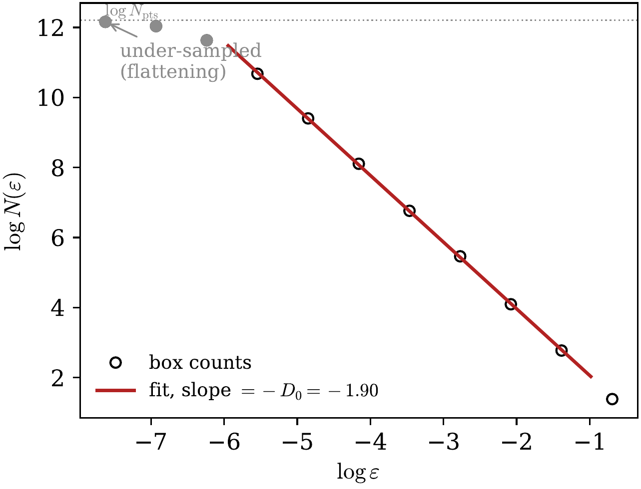
Figure 7.5 Determination of the box-counting dimension from the slope of \(\log N(\varepsilon)\) against \(\log\varepsilon\).#
The same procedure applies without modification to the strange attractors of the previous chapters, since a Poincaré section turns a continuous flow into a cloud of points in the plane. Applied to the Lorenz attractor it returns a dimension slightly above two, confirming the non-integer dimension anticipated in chapter 6 and resolving the volume-contraction paradox with which this chapter opened.
7.3. The correlation dimension#
The box-counting method treats all occupied boxes on the same footing, whether a box contains a single point or a thousand. For experimental attractors it is often more robust to characterize the object through the density of pairs of points that lie close together. This leads to the correlation dimension.
For a set of \(N\) points \(\mathbf{x}_1,\ldots,\mathbf{x}_N\) one defines the correlation integral
where \(\Theta\) is the Heaviside step function. In words, \(C(r)\) is the fraction of all pairs of points whose separation is smaller than \(r\). If the points are distributed on a fractal object, the number of neighbours within a distance \(r\) of a given point scales as \(r^{D_2}\), so that
which defines the correlation dimension
As with box-counting, \(D_2\) is estimated in practice from the slope of a \(\log C(r)\) versus \(\log r\) plot over the scaling range. The correlation dimension is generally somewhat smaller than the box-counting dimension, \(D_2 \leq D_0\), with equality only when the points are uniformly distributed over the object; it is the member \(q=2\) of the family of generalized dimensions.
The following maple fragment computes the correlation integral for a set of \(N\) points \((x_n,y_n)\). Rather than sorting distances, the pairwise separations are binned logarithmically between \(r_{\min}\) and \(r_{\max}\), and the bins are accumulated to form the cumulative count \(C(r)\).
Maple
restart; with(plots):
# ... x, y and N are assumed to hold the data set ...
rmin := 0.04: rmax := 5.0: M := 20:
mumin := log(rmin): mumax := log(rmax):
dmu := (mumax - mumin)/M:
for m from 0 to M do
  cor[m]   := 0;
  scale[m] := exp(mumin + dmu*(m + 0.5));   # representative r of bin m
end do:
for i from 2 to N do                        # loop over all pairs i>j
  for j from 1 to i-1 do
    distance := sqrt((x[i]-x[j])^2 + (y[i]-y[j])^2);
    m := trunc((log(distance + 1e-10) - mumin)/dmu);
    if (m >= 0 and m <= M) then cor[m] := cor[m] + 1; end if;
  end do:
end do:
for m from 1 to M do
  cor[m] := cor[m] + cor[m-1];              # cumulative -> C(r)
end do:
loli := seq([log(scale[m]), log(cor[m])], m=1..M):
The slope of a straight-line fit to loli yields the correlation dimension \(D_2\) directly. Applied to the dripping-faucet attractors, this procedure gives values close to, but slightly below, the box-counting dimensions of section 7.2, consistent with the general ordering \(D_2\leq D_0\).
7.4. Multifractals and generalized dimensions#
So far we have characterized a fractal object by a single number, its dimension. This is adequate when the points are distributed more or less uniformly over the object. Many attractors, however, are highly non-uniform: the trajectory spends far more time in some regions than in others, so that the measure is concentrated in a way that a purely geometric dimension cannot capture. Such objects are called multifractals, and their proper description requires not one dimension but a whole spectrum.
To make this quantitative, we cover the object with boxes of size \(\varepsilon\) as before, but now we keep track of the fraction \(p_i(\varepsilon)\) of the total measure that falls in box \(i\) (for a time series, \(p_i\) is the fraction of time the trajectory spends in box \(i\)). We then form the partition sum
where the sum runs over occupied boxes and \(q\) is a real parameter. Positive values of \(q\) emphasize the densely populated boxes, whereas negative values of \(q\) emphasize the sparsely populated ones. In analogy with (7.6) one expects a power-law scaling \(Z(q,\varepsilon)\sim \varepsilon^{(q-1)D_q}\) and defines the generalized dimension of order \(q\) as
The prefactor \(1/(q-1)\) is chosen so that \(D_q\) reproduces the dimensions we already know for the special values of \(q\):
For \(q=0\), \(\sum_i p_i^{0}\) simply counts the number of occupied boxes \(N(\varepsilon)\), so that \(D_0\) is the box-counting dimension (7.7).
For \(q=2\), \(\sum_i p_i^{2}\) is the probability that two randomly chosen points fall in the same box, and \(D_2\) is the correlation dimension (7.10).
For \(q\rightarrow 1\) the definition becomes indeterminate; taking the limit carefully (l'Hôpital) yields the information dimension
in which the numerator is (minus) the Shannon entropy of the box distribution.
The generalized dimensions form a non-increasing sequence, \(D_q \geq D_{q'}\) for \(q<q'\). For a monofractal, where the measure is spread uniformly, all \(D_q\) are equal and the spectrum collapses to a single value. A genuine multifractal has a \(D_q\) that decreases with \(q\): the width of the spectrum \(D_{-\infty}-D_{+\infty}\) measures how non-uniform the object is.
7.4.1. A binomial multifractal#
The mechanism is best understood through an explicit construction. Consider the unit interval carrying a unit of “mass”. At the first step we split the interval into two equal halves and distribute the mass in the proportion \(p_1\) to the left half and \(p_2 = 1-p_1\) to the right half. At the second step each half is again split in two and its mass redistributed in the same proportion \(p_1 : p_2\), and so on. After \(k\) steps the interval has been divided into \(2^{k}\) sub-intervals of length \(\varepsilon = 2^{-k}\), and the measure contained in a sub-interval reached through a particular sequence of left/right choices is a product of the form
where \(m\) is the number of times the “left” branch was taken. This recursive assignment,
generates a self-similar measure on the interval (Figure 7.6). For \(p_1=p_2=\tfrac12\) the mass is spread uniformly and the object is monofractal, but for \(p_1\neq p_2\) it becomes increasingly spiky as \(k\) grows, with the bulk of the measure concentrated on a vanishingly small fraction of the interval.
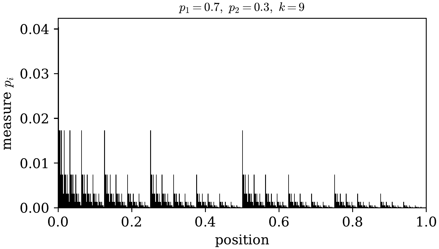
Figure 7.6 A binomial multifractal measure obtained by repeatedly redistributing the mass of each sub-interval in the ratio \(p_1:p_2\).#
The generalized dimensions of this measure can be obtained analytically. Because the \(2^{k}\) sub-intervals realize every combination of left/right choices, the partition sum (7.11) factorizes,
where the last step uses the binomial theorem. With \(\varepsilon = 2^{-k}\) we have \(\log\varepsilon = -k\log 2\), and substitution into (7.12) gives the closed-form result
One verifies immediately that \(D_0 = \log 2/\log 2 = 1\): the measure lives on the whole interval, so the support is one-dimensional. The information about the non-uniformity is carried entirely by the dependence of \(D_q\) on \(q\). For \(p_1=p_2=\tfrac12\) equation (7.14) gives \(D_q = 1\) for all \(q\) (monofractal), whereas for \(p_1\neq p_2\) the dimension \(D_q\) decreases monotonically from \(D_{-\infty}\) to \(D_{+\infty}\), producing the characteristic sigmoidal \(D_q\) curve of Figure 7.7.
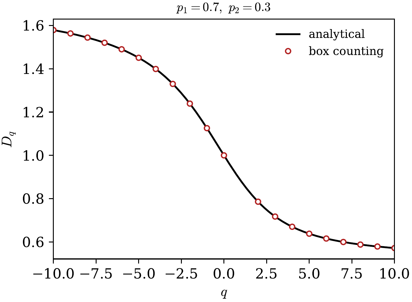
Figure 7.7 The generalized-dimension spectrum \(D_q\) of the binomial multifractal, comparing the analytical result with the box-counting procedure.#
7.4.2. Numerical determination of \(D_q\)#
The generalized dimensions of an arbitrary measure are computed by a straightforward extension of the box-counting algorithm. For each box size \(\varepsilon = 2^{-p}\) one accumulates the measure \(p_i\) in every box, forms the partition sum \(Z(q,\varepsilon)=\sum_i p_i^{q}\), and records \(\log Z\) against \(\log\varepsilon\). Repeating this over a range of box sizes and fitting a straight line gives the slope, from which \(D_q = \text{slope}/(q-1)\) follows for each \(q\).
Maple
restart: with(stats):
read "p1p2.dat":                         # loads the measure dat[1..N]
N := nops(dat);
x := [seq(n/N, n=1..N)]:
listDq := NULL:
for q from -10 to 10 do
  if q = 1 then next; end if;            # q=1 is singular, skip it
  loli := NULL:
  for p from 2 to 9 do
    delta := 1.0/2^p;
    nb := 2^p;
    nr := Array(1..nb, 0.0);
    for n from 1 to N do                 # bin the measure
      i := trunc(x[n]/delta) + 1;
      nr[i] := nr[i] + dat[n];
    end do:
    Z := add(`if`(nr[i] > 0, nr[i]^q, 0), i=1..nb);
    loli := loli, [log(delta), log(Z)];
  end do:
  xli := [seq(loli[k][1], k=1..nops([loli]))]:
  yli := [seq(loli[k][2], k=1..nops([loli]))]:
  eq  := fit[leastsquare[[x,y], y=a*x+b]]([xli, yli]);
  Dq  := coeff(rhs(eq), x)/(q-1);        # slope / (q-1)
  listDq := listDq, [q, Dq];
end do:
plot([listDq], labels=["q","D(q)"]);
The value \(q=1\) is skipped in the loop because of the \(1/(q-1)\) singularity; the information dimension (7.13) would have to be evaluated separately. Comparing the numerical spectrum with the analytical expression (7.14) (Figure 7.7) provides a stringent test of the box-counting implementation, and shows the same under-sampling limitations at large \(|q|\) that we encountered for \(D_0\): extreme values of \(q\) weight either the most or the least populated boxes, both of which are the most poorly sampled.
Example
The construction generalizes to any number of branches. Splitting each interval into three parts with weights \(p_1,p_2,p_3\) leads, by the same argument, to
Setting one of the weights to zero prunes the corresponding branch at every stage, and the support of the measure becomes a Cantor-like dust rather than the full interval. For instance, with \(p_2=0\) and \(p_1=p_3=\tfrac12\) the measure is uniform on the two surviving thirds, and (7.15) reduces for \(q=0\) to \(D_0 = \log 2/\log 3\), exactly the dimension (7.4) of the middle-third Cantor set. Choosing instead \(p_2=0\), \(p_1=\tfrac45\), \(p_3=\tfrac15\) gives a genuine multifractal supported on the Cantor set, whose spectrum \(D_q\) again follows (7.15).
Fractal geometry of turbulence
Fractals are not merely mathematical constructions; turbulent flows produce them in abundance. A striking example is the turbulent/non-turbulent interface (TNTI), the sharp but intricately folded surface that separates the rotational, turbulent fluid in a jet, wake or gravity current from the irrotational fluid around it [Corrsin and Kistler, 1954]. It is convoluted across the whole range of eddy sizes, from the integral scale \(l_o\) down to a few Kolmogorov lengths \(l_i\), and box-counting (section 7.2) of the interface area yields a power law [Mandelbrot, 1982, Sreenivasan et al., 1989]
where \(D_f\) is the fractal dimension of the surface. A planar cut through it is a fractal curve whose length scales as \(L(\lambda)\propto \lambda^{-\beta}\) with \(\beta = D_f-2\); high-Reynolds-number flows give \(\beta \approx 1/3\), i.e. \(D_f\approx 7/3\) [de Silva et al., 2013, Sreenivasan, 1991]. This matters because the interface area controls entrainment: the more convoluted the interface, the faster the turbulence engulfs and mixes the surrounding fluid.
What sets \(\beta\)? A self-similar model in the spirit of section 7.1 is revealing (Figure 7.8). A segment of length \(l_n\) is replaced by two segments meeting at a vertex displaced a distance \(r\,l_n\) off its midpoint, the side alternating so that the mean position is preserved. Each new segment has length \(l_{n+1} = \tfrac12 m\, l_n\) with \(m=\sqrt{1+4r^2}\), and there are twice as many, so the curve consists of \(N=2\) copies of itself scaled by \(s=m/2\). Its dimension then follows straight from the similarity dimension (7.2),
This is the von Koch construction with a tunable bump: \(r\approx 0.32\) reproduces \(\beta=1/3\), whereas smaller \(r\) gives a flatter, lower-dimensional interface.
The anisotropy parameter \(r\) – the height of the interface bulges relative to their width – is where the physics enters. In a stratified gravity current a stable density gradient suppresses the vertical excursions of the interface while its streamwise extent stays fixed by the shear layer, so \(r\) decreases as the stratification (measured by the Richardson number) grows. Through the relation above this lowers \(\beta\), shrinks the interface area \(A_\eta\), and throttles the entrainment of ambient fluid [Krug et al., 2017]; in the limit \(\beta\to0\) the interface becomes smooth and mixing collapses to molecular diffusion. The fractal dimension is thus a genuine control parameter for turbulent mixing in the ocean and atmosphere. (Should \(r\) itself vary with scale, the interface is no longer a simple fractal but a multifractal of the kind met in section 7.4.)
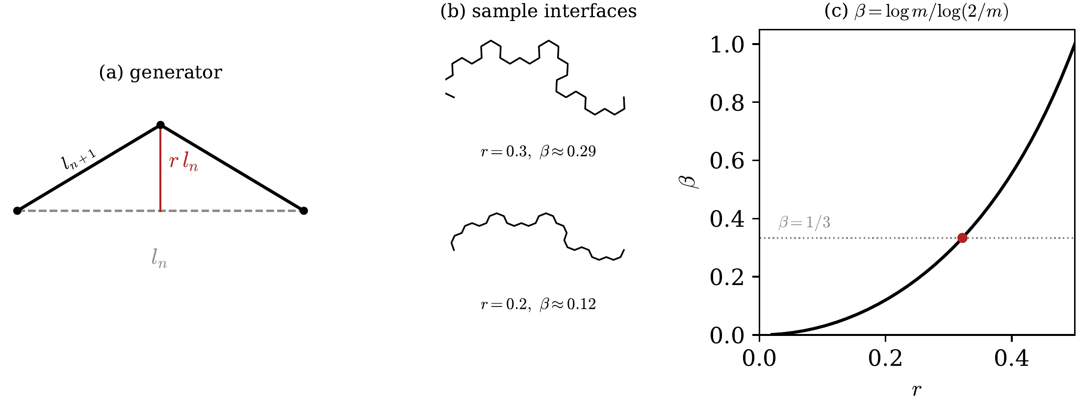
Figure 7.8 A self-similar model of the turbulent/non-turbulent interface [Krug2017]. (a) The generator: a segment of length \(l_n\) is replaced by two segments meeting at a vertex displaced by \(r\,l_n\) off the midpoint. (b) Curves after five iterations for \(r=0.3\) and \(r=0.2\); the smaller \(r\) produces a smoother, lower-dimensional interface. (c) The fractal exponent \(\beta = \log m/\log(2/m)\) as a function of the anisotropy \(r\), with the neutral-turbulence value \(\beta=1/3\) marked.#
Fractal clouds
The boundary of a cumulus cloud is one of the most familiar fractals in Nature. Satellite images show that the cloud perimeter has a fractal dimension close to \(4/3\) over four orders of magnitude in size which, assuming isotropy, means the cloud surface scales as \(A\sim L^{D_s}\) with \(D_s\simeq 7/3\). Siebesma and Jonker [2000] tested this with a computer model of the atmosphere (a large-eddy simulation) and measured the dimension of individual simulated clouds using exactly the tools of this chapter: the volume–surface scaling \(A\sim L^{D_s}\) and the correlation integral (7.8). Both gave \(D_s = 2.3\ldots\), in striking agreement with the observations (Figure 7.9).
The value \(7/3\) is no accident. It is precisely the surface dimension for which the turbulent transport of heat and moisture across the (unresolved) cloud edge becomes independent of the grid resolution – so it is the fractal geometry of the interface that makes the mixing, or entrainment, come out right. The fractal cloud boundary is really the turbulent/non-turbulent interface of the previous box, now seen from the sky.
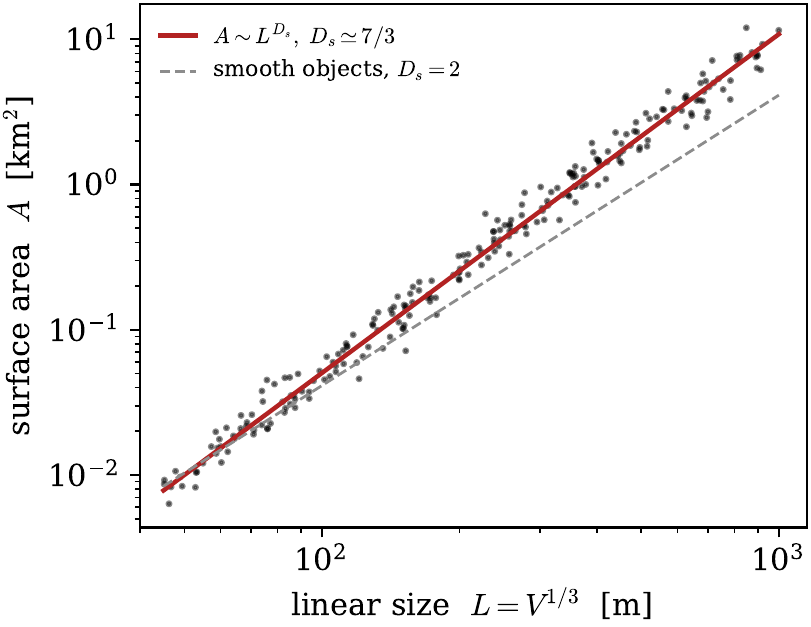
Figure 7.9 Surface area \(A\) against linear size \(L=V^{1/3}\) for a population of simulated cumulus clouds (schematic, after Siebesma & Jonker, 2000). The clouds obey \(A\sim L^{D_s}\) with \(D_s\simeq 7/3\) (solid line), well above the \(D_s=2\) of smooth, Euclidean shapes (dashed line).#
7.5. Exercises#
7.5.1. Correlation dimension#
Downloads: CorrelationDimension.mws
a) Write a maple program to calculate the correlation dimension of a set consisting of \(N\) points \((x_n,y_n)\).
b) Calculate the correlation dimension of the dripping faucet attractors and compare the values with the box-dimension.
7.5.2. Fractal Properties of the Forced Double Well Oscillator#
Downloads: DoubleWellFractal.mws, DoubleWellFractal_start.mws, ex0121r00_fig1.eps, ex0121r00_fig2.eps
Consider a slender steel beam with a damping coefficient \(f\) that is clamped in a rigid framework (Figure 7.10). Two permanent magnets at the base pull the beam in opposite directions and the magnets are so strong that the beam buckles to one side or the other. The system is driven out of its equilibrium by shaking it with angular frequency \(\omega\) and force \(A\).
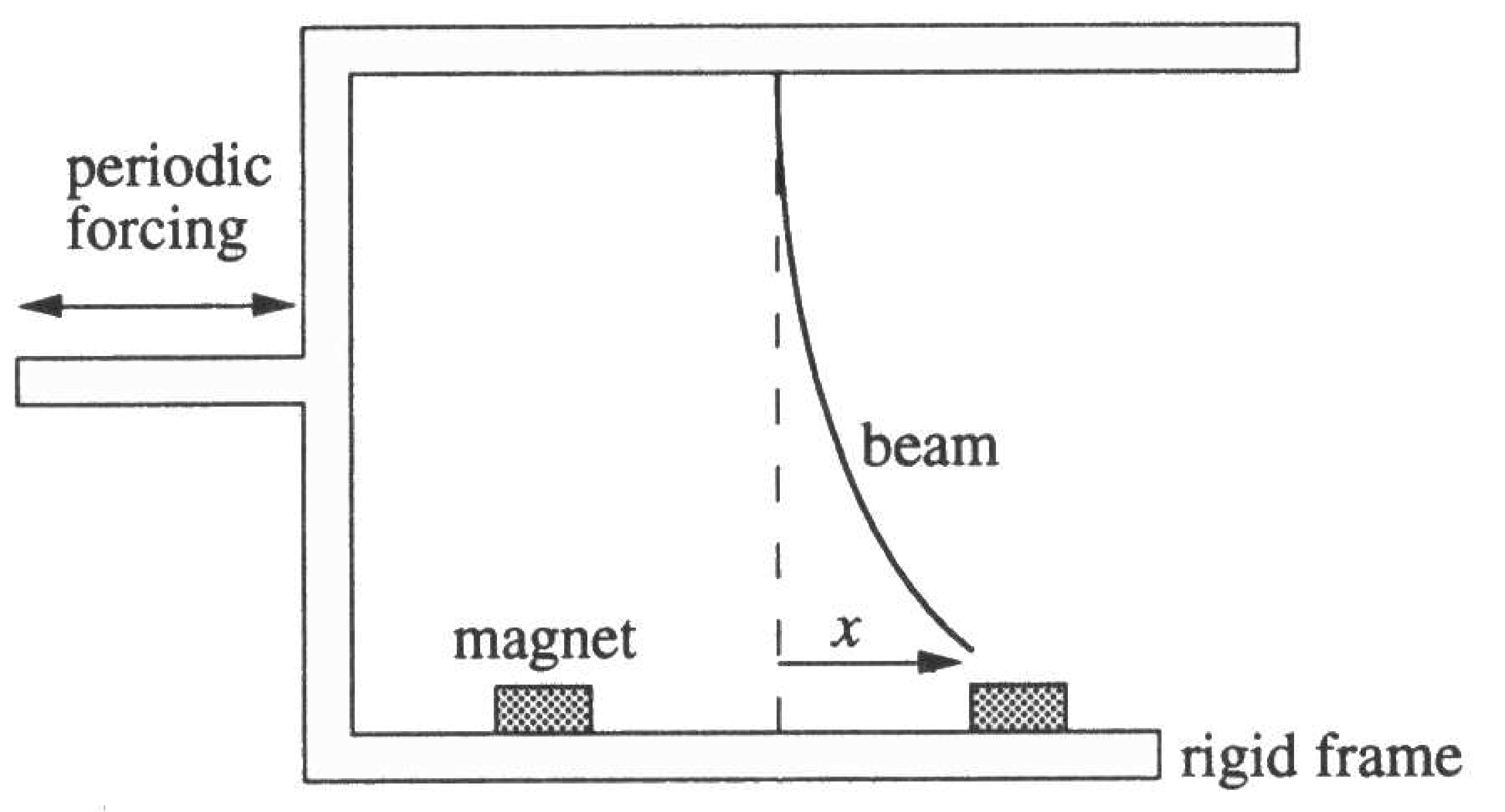
Figure 7.10 Sketch of the mechanical system.#
Written as an autonomous system of first order nonlinear differential equations, the system's behavior is defined by
a) Open the file DoubleWellFractal_start.mws, and execute it for \(A=0.3\). This generates output like shown in Figure 7.11. What does this code-fragment do? What is the name of this plotting method? Why and when would this be useful?
b) Determine the box-dimension of this attractor.
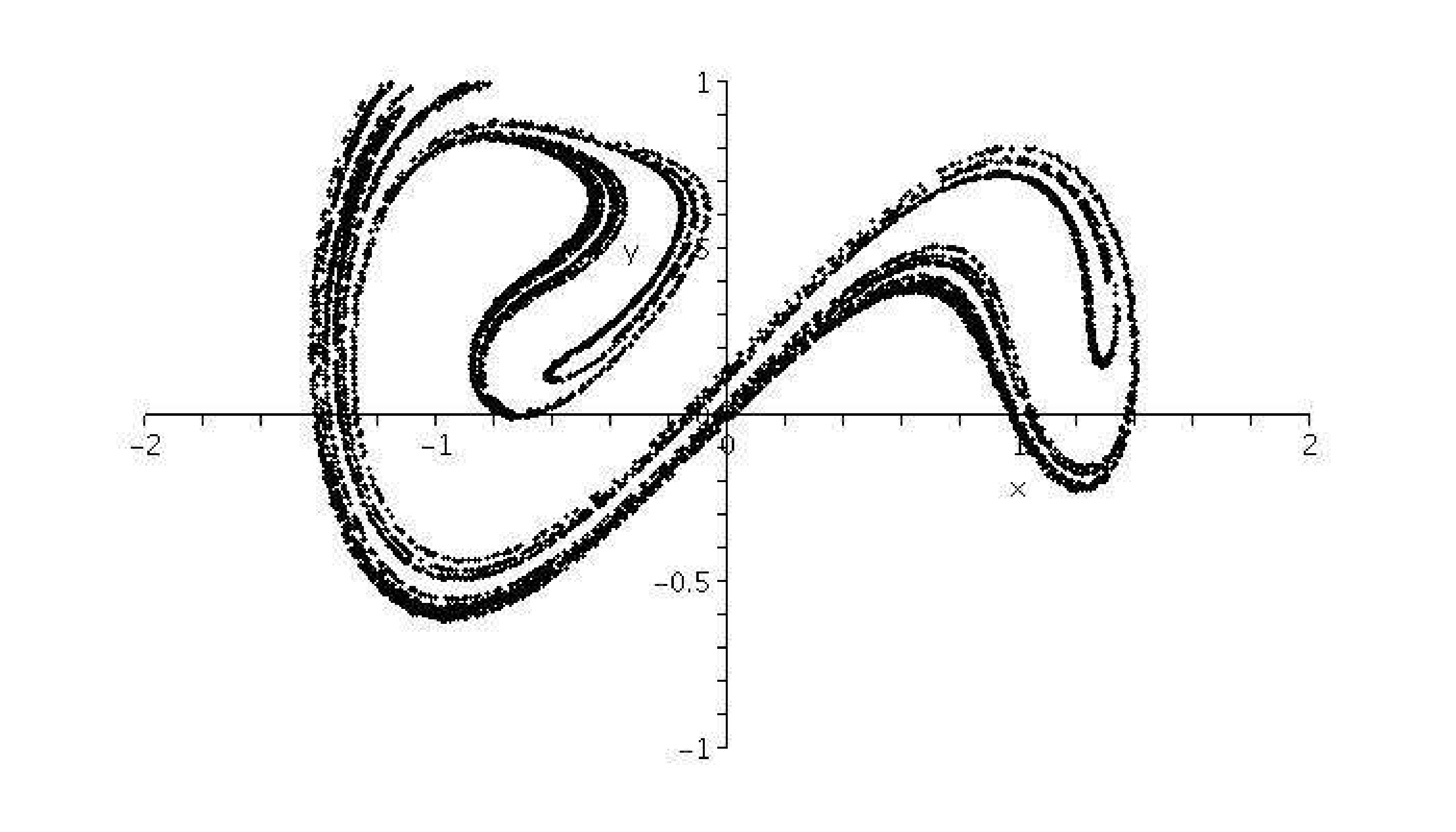
Figure 7.11 Result from executing DoubleWellFractal\_start.mws with \(N=10000\).#
7.5.3. Fractal Curve#
Downloads: FractalCurve.mws, FractalCurve.data, FractalCurve_start.mws, FractalCurve_creator.mws, FractalCurve.eps
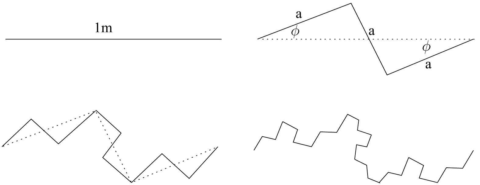
Figure 7.12 Fractal Curve generation: first four recursive steps#
Consider the above sketched recursive generation of a family of fractal curves parameterized by \(\phi\), with \(0 \leq \phi \leq \pi/6\). Note that the three segments have equal size \(a=a(\phi)\) and that \(a\cos(\phi) \leq 1/2\).
a) Express the fractal dimension \(d\) of the curve in terms of \(\phi\) and plot the result.
b) Take \(\phi = \pi/7\). After how many recursive steps is the length of the curve larger than 1km?
c) The file FractalCurve.data contains the points of a certain curve generated along the way outline above. Open the maple file FractalCurve_start.mws which reads this data set, and calculate the curve's fractal dimension using the box-counting method.
7.5.4. Multi-fractals in threes#
Downloads: MultifractalThree.mws
a) Generate a multi-fractal set with \(N=3^6\) points, according to the formalism: \([1]\rightarrow [p_1,p_2,p_3] \rightarrow [p_{1}^{2}, p_{1}p_{2}, p_{1}p_{3}, \,p_{1}p_{2}, p_{2}^{2}, p_{2}p_{3}, \,p_{1}p_{3}, p_{2}p_{3}, p_{3}^{2}] \rightarrow \ldots\).
b) Take \(p_{2} = 0\), and \(p_{3} = p_{1} = 1/2\). Calculate analytically the fractal dimension (the box dimension).
c) Take \(p_{2} = 0\), \(p_{1} = 4/5\) and \(p_{3} = 1/5\). Calculate analytically the generalized dimension \(D(q)\).
d) Take \(p_{2} = 0\), \(p_{1} = 4/5\) and \(p_{3} = 1/5\). Calculate the generalized dimension \(D(q)\) by the box-counting procedure for \(q\) in the range \(q \in [-10,10]\) (avoid calculating \(q=1\) in the procedure). Plot the result and compare the outcome with the analytical result obtained in (c). (Hint: divide the boxes each time in three parts.)