8. Chaos in practice#
The book began with a paradox – that simple, entirely deterministic equations can produce behaviour that is impossible to predict in the long run – and has since assembled the geometric machinery needed to understand it: phase space and flows, fixed points and their stability, bifurcations and the routes to chaos, Lyapunov exponents, strange attractors and, in the previous chapter, their fractal geometry. All of this was developed on deliberately small systems, from one-dimensional maps to the three equations of Lorenz, precisely so that every idea could be computed and drawn.
The purpose of this final chapter is to look outward. The same handful of concepts – a finite horizon of predictability, a cloud of trajectories in place of a single one, an attractor of far lower dimension than the space it lives in – are not merely of historical interest. They are the working machinery of modern computational science, from weather forecasting and climate reanalysis to the reduced-order modelling of turbulence and the analysis of measured signals. We shall introduce no new mathematics. Instead we show that the reader has acquired a way of thinking about nonlinear systems, and follow it along two complementary lines. Because prediction has a finite horizon, we must predict with ensembles, correct with data, and reduce with structure; and where chaos is an asset rather than an obstacle, we can turn it to advantage – to mix, to control, and to reconstruct. Throughout, the Lorenz equations of chapter 6 serve as a concrete laboratory in which each idea can still be run on a desktop.
8.1. Prediction in an uncertain world#
It is worth pausing to see why a weather forecast belongs in this book at all. A numerical weather model solves the equations of motion of the atmosphere – conservation of mass, momentum and energy for a rotating, stratified, moist fluid – on a grid covering the globe. Collecting every field value (three velocity components, temperature, pressure, humidity, …) at every grid point into a single enormous column vector \(\mathbf{x}\), the model is nothing other than a system of ordinary differential equations
of exactly the form (6.1) that we have studied since chapter 5. The only difference is one of scale: where the Lorenz system has three components, a modern forecast model has a state vector \(\mathbf{x}\) whose dimension is of order \(10^{9}\) (Figure 8.1).
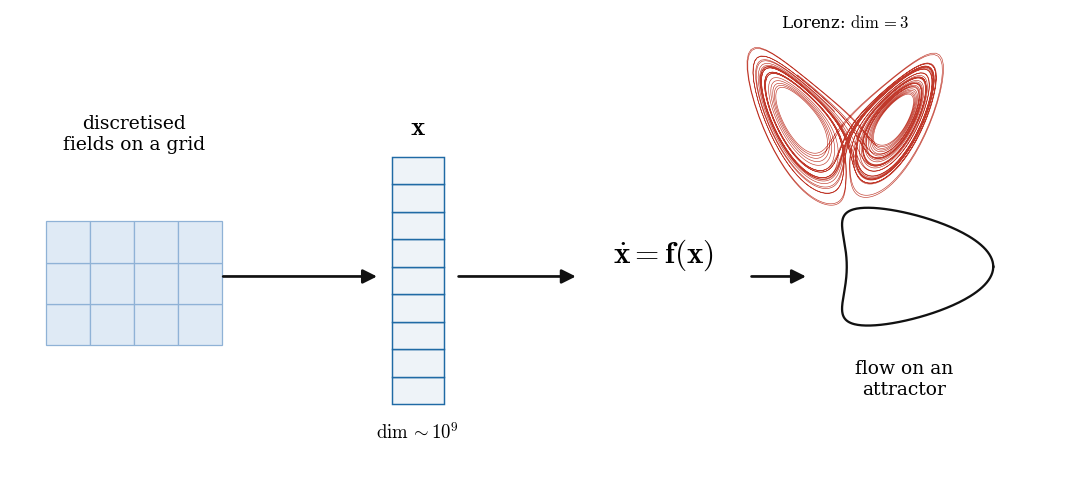
Figure 8.1 A weather model is a dynamical system. The discretised atmospheric fields are stacked into one state vector \(\mathbf{x}\) of dimension of order \(10^{9}\), whose evolution obeys \(\dot{\mathbf{x}} = \mathbf{f}(\mathbf{x})\). The Lorenz system is the same kind of object at the opposite extreme of dimension.#
This is more than an analogy. As shown in appendix 2, the Lorenz equations were themselves obtained by Galerkin-truncating a convection model until only three modes remained. The tiny system the reader now knows intimately and the billion-dimensional weather model are therefore the same construction seen at two extremes of dimension. Everything the book has established about (8.1) carries over: the forced–dissipative atmosphere is drawn onto an attractor – the climate – on which the ever-changing weather is nothing but the trajectory itself; the motion on that attractor has a positive Lyapunov exponent, and hence a sensitive dependence on initial conditions. It was in contemplating exactly this that Lorenz was led to his three equations, and it is this that makes weather prediction hard. The rest of the chapter simply pushes the familiar ideas up in dimension.
The first of these ideas concerns the limits of prediction. The central lesson of chaos is not that prediction is impossible, but that every prediction has a finite horizon. Two trajectories that start a distance \(\delta_0\) apart separate, on average, as \(\delta(t) \sim \delta_0\, \mathrm{e}^{\Lambda_e t}\), where \(\Lambda_e\) is the effective Lyapunov exponent of chapter 6. A forecast remains useful only until this error grows to the size of the attractor itself. For the Lorenz system, with \(\Lambda_e \approx 0.9\) (section 6.1), an initial uncertainty of \(\delta_0 = 10^{-3}\) grows to order ten in a time
after which the forecast retains no information about the specific initial condition. The atmosphere behaves in exactly the same way; it is only the numbers that differ, giving the familiar horizon of a week or two for weather. Its effective growth rate is not a single constant, however, but varies with the flow regime and with the spatial scale of the feature one is trying to predict, so this horizon is itself only a typical value.
Since the initial state is never known exactly, the honest response is to abandon the single deterministic forecast and to propagate instead a whole cloud of initial conditions, each an equally plausible estimate of the true state. This is the idea of ensemble forecasting. Rather than one trajectory, one integrates many, and reads off the forecast not as a single number but as the distribution of the ensemble. The butterfly effect thereby ceases to be a curiosity and becomes an operational quantity: the spread of the ensemble is the forecast's own estimate of its uncertainty.
Figure 8.2 shows a Lorenz ensemble: a tight blob of initial conditions is stretched into a filament along the attractor and, by \(t=8\), smeared across it entirely. The blob's growth is quantified in Figure 8.3, which tracks the ensemble spread \(\delta(t)\). It grows exponentially at the rate \(\Lambda_e = 0.9\) set by the Lyapunov analysis, until it saturates at the size of the attractor. The time at which the spread becomes an appreciable fraction of the attractor is the predictability horizon: beyond it, the ensemble members are effectively uncorrelated and only the climatological distribution remains.
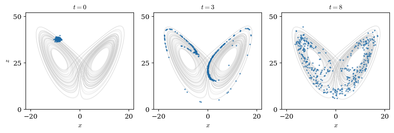
Figure 8.2 An ensemble forecast for the Lorenz system, shown in the \((x,z)\) projection. A tight blob of initial conditions (left) is stretched into a filament by the flow, and eventually spread over the whole attractor. The width of the cloud is the forecast uncertainty.#
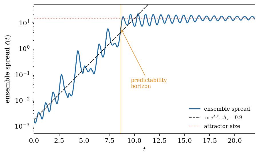
Figure 8.3 Growth of the ensemble spread \(\delta(t)\) for the blob of Figure 8.2. The spread grows as \(\mathrm{e}^{\Lambda_e t}\) with \(\Lambda_e = 0.9\) (dashed) until it saturates at the size of the attractor (dotted). The predictability horizon is reached when the two meet.#
Maple
The ensemble is generated by integrating the Lorenz equations from a set of perturbed initial conditions and measuring how the cloud spreads. Starting from a point x0 already on the attractor (obtained as in chapter 6 by discarding a transient), we draw M nearby initial conditions and integrate each.
restart; with(Statistics): with(LinearAlgebra):
sigma := 10: r := 28: b := 8/3:
DE := diff(x(t),t) = sigma*(y(t)-x(t)),
      diff(y(t),t) = r*x(t) - y(t) - x(t)*z(t),
      diff(z(t),t) = x(t)*y(t) - b*z(t):

M     := 400:                                   # ensemble size
eps0  := 1e-3:                                  # initial spread
for m from 1 to M do                            # perturb the initial state
  ic := x(0)=x0[1]+eps0*Sample(Normal(0,1),1)[1],
        y(0)=x0[2]+eps0*Sample(Normal(0,1),1)[1],
        z(0)=x0[3]+eps0*Sample(Normal(0,1),1)[1];
  sol[m] := dsolve({DE, ic}, numeric, output=listprocedure):
end do:

for i from 1 to N do                            # spread at each time t[i]
  cloud := Matrix(M, 3):
  for m from 1 to M do
    cloud[m,1] := eval(x(t), sol[m])(t[i]);
    cloud[m,2] := eval(y(t), sol[m])(t[i]);
    cloud[m,3] := eval(z(t), sol[m])(t[i]);
  end do:
  cbar     := <Mean(cloud[..,1]), Mean(cloud[..,2]), Mean(cloud[..,3])>;
  delta[i] := sqrt(add(Norm(<cloud[m,1..3]> - cbar, 2)^2, m=1..M)/M);
end do:
Ensemble weather forecasting
Operational weather centres run precisely this calculation, but with \(\dim\mathbf{x}\sim 10^{9}\) instead of three. Because one cannot integrate millions of members, a modest ensemble of some 50 forecasts is launched from slightly perturbed initial conditions and slightly perturbed model physics [Bauer et al., 2015, Lorenz, 1996]. The spread of the ensemble at a given lead time is the forecast uncertainty: when the members agree, the forecast is confident; when they diverge, it is not. This is how a probability of rain is produced, and it is why forecasts now come with a horizon attached. The transformation of weather prediction from a single deterministic run into a routine estimate of its own uncertainty has been called a quiet revolution [Bauer et al., 2015]; at its root lies nothing more than the sensitive dependence on initial conditions of chapter 6.
8.2. Observations and models: data assimilation#
A forecast needs a starting point, and here a second difficulty appears: the true state \(\mathbf{x}\) is never known. We have instead a stream of noisy, incomplete observations – a scatter of measurements that constrains the state without determining it. Forecasting in practice is therefore a continuous cycle: predict the state forward with the model, observe it where measurements are available, and correct the prediction towards the observations, before predicting again. Combining a model with data in this way is called data assimilation, and it is once more an application of the dynamical system (8.1).
The classical tool for the correction step is the Kalman filter [Kalman, 1960]. Its central idea is disarmingly simple: the corrected estimate, called the analysis, is a weighted average of the model forecast and the observation,
where \(\mathbf{x}_f\) is the forecast, \(\mathbf{y}\) the observation, and \(H\) the operator that maps a state to the quantities actually measured. The quantity \(\mathbf{y} - H\mathbf{x}_f\) is the innovation, the amount by which the observation surprises the forecast, and the Kalman gain \(K\) is the weight applied to it. The gain is chosen by the relative confidence in model and data: writing \(P\) for the covariance (the uncertainty) of the forecast and \(R\) for that of the observations,
When the observations are precise (\(R\) small) the gain is large and the analysis follows the data; when the model is trusted (\(P\) small) the gain is small and the analysis stays close to the forecast. The filter alternates two steps: a forecast step, in which both the state and its uncertainty \(P\) are advanced by the model, and an update step (8.2)–(8.3), in which the incoming observation shrinks that uncertainty.
Advancing the uncertainty is the only subtlety. The textbook Kalman filter is linear, whereas \(\mathbf{f}\) is not, so the covariance is propagated through the linearisation of the flow – and that linearisation is precisely the Jacobian \(J\) already used to compute the Lyapunov exponents in chapter 6. This is the extended Kalman filter. No new machinery is needed: over one assimilation window the forecast covariance evolves as \(P_f = \Phi\, P_a\, \Phi^{\top} + Q\), where the state-transition matrix \(\Phi\) is obtained by integrating \(\dot{\Phi} = J\,\Phi\) with \(\Phi(0)=I\), and \(Q\) accounts for imperfections in the model.
Figure 8.4 shows the result of a twin experiment on the Lorenz system: we integrate a "truth" trajectory, generate noisy observations from it, and then try to recover it from a deliberately wrong initial guess. A free forecast, left to run without corrections, diverges from the truth within the predictability horizon of the previous section. The Kalman filter, fed the same noisy observations, locks onto the truth and tracks it indefinitely, its error held an order of magnitude below the free run. The finite horizon has not been abolished – it cannot be – but by repeatedly injecting information it is continually reset before the error can grow to saturation.
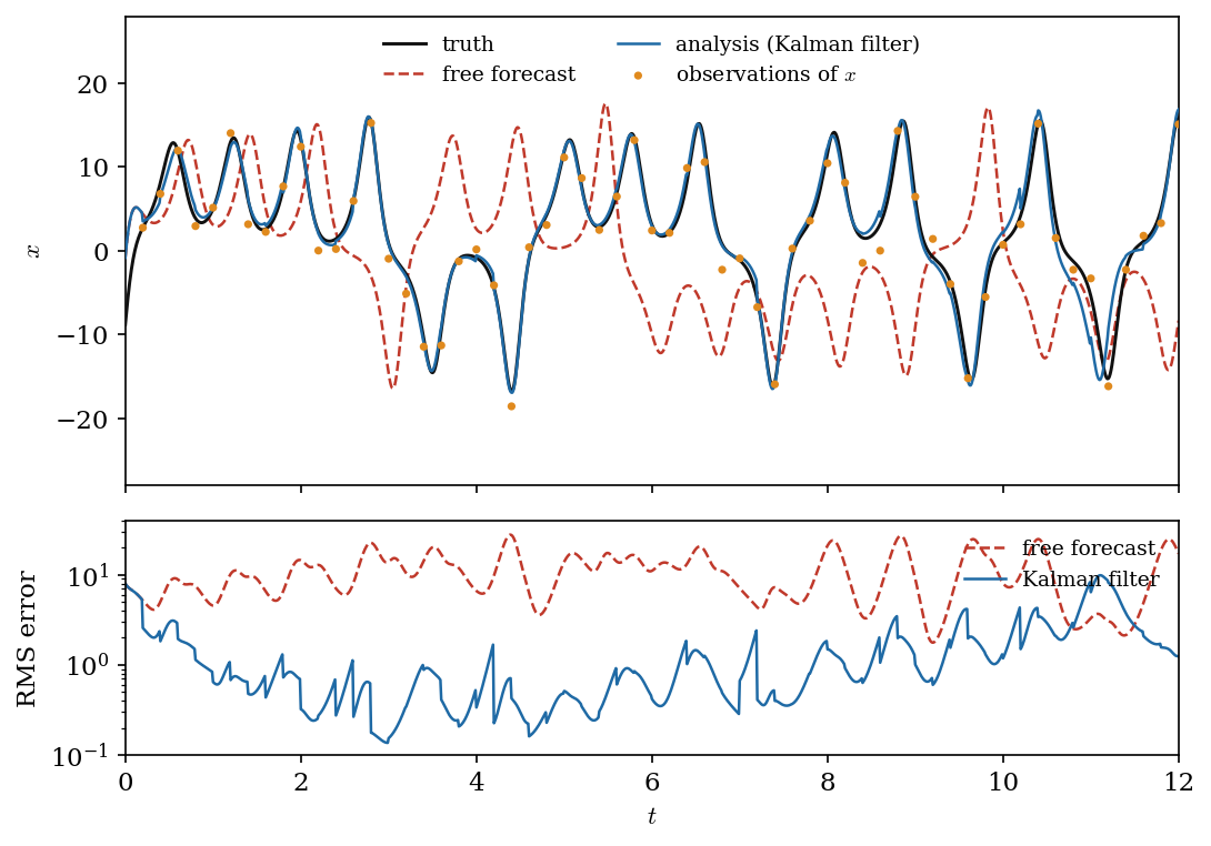
Figure 8.4 Data assimilation for the Lorenz system. Top: the \(x\)-component of the truth, a free forecast started from a wrong initial condition, and the Kalman-filter analysis fed noisy observations (dots). Bottom: the RMS error of the two estimates. The free forecast diverges within the predictability horizon; the analysis stays locked on.#
Maple
The filter is a short loop over the observation times. Between observations the state is advanced with dsolve and the covariance with the Jacobian Jac; at each observation the analysis and its covariance are updated using the Kalman gain (8.3). The Jacobian is the same one used for the Lyapunov exponents in chapter 6.
restart; with(LinearAlgebra):
sigma := 10: r := 28: b := 8/3:
f   := (x,y,z) -> <sigma*(y-x), r*x - y - x*z, x*y - b*z>:
Jac := (x,y,z) -> <<-sigma, r-z,  y> |
                   < sigma,  -1,  x> |
                   <  0,     -x, -b>>:              # as in chapter cont3d

H  := IdentityMatrix(3):                            # full state observed
R  := (1.5)^2 * IdentityMatrix(3):                  # observation error
Q  := 0.01   * IdentityMatrix(3):                   # model error
I3 := IdentityMatrix(3):

xa := <-5.0, -5.0, 25.0>:                           # wrong first guess
Pa := 4.0 * IdentityMatrix(3):                      # its uncertainty

for k from 1 to Nobs do
  # --- forecast: advance state and covariance over one window ---
  xf  := advance(xa, dtobs):                        # integrate the ODE
  Phi := transition(xa, dtobs):                     # solve d(Phi)/dt = Jac.Phi
  Pf  := 1.03 * Phi . Pa . Transpose(Phi) + Q:      # (mild inflation)
  # --- update: blend the forecast with observation y[k] ---
  S  := H . Pf . Transpose(H) + R:
  K  := Pf . Transpose(H) . MatrixInverse(S):       # Kalman gain
  xa := xf + K . (y[k] - H . xf):                   # analysis
  Pa := (I3 - K . H) . Pf:                          # reduced uncertainty
  Xa[k] := xa:
end do:
Because the Lorenz system has only three variables, its error covariance \(P\) is a \(3\times 3\) matrix that can be stored and propagated exactly. This is what makes the example transparent, but it is also exactly what is impossible in an operational model, where \(P\) would be a \(10^{9}\times 10^{9}\) matrix that can be neither stored nor propagated. The extended Kalman filter is thus the natural nonlinear extension in principle but is unusable for global forecasting in practice, and overcoming this is the central technical problem of modern data assimilation. Two families of practical methods have emerged. Ensemble methods replace the explicit covariance with the sample covariance of a modest ensemble (section 8.1), giving the ensemble Kalman filter [Evensen, 2003], supplemented by localisation and inflation to control sampling error. Variational methods, on which the major operational centres principally rely, instead fit the model trajectory to a whole window of observations by numerical optimisation (the technique known as 4D-Var), and are increasingly combined with ensembles into hybrid schemes [Bauer et al., 2015]. The Kalman filter of (8.2) is best regarded as the conceptual prototype for all of these rather than the operational algorithm itself; what they share is unchanged from it – predict, observe, and correct in proportion to confidence.
Run this same cycle continuously on a model of one specific engineered system – an aircraft engine, a bridge, a patient's circulation – kept synchronised to its physical counterpart by a live stream of sensor data, and one has what engineering now calls a digital twin: data assimilation applied not to the planet but to a single machine, and often accelerated by the reduced-order surrogates of the next section.
Reanalysis: replaying the atmosphere
Apply the same assimilation cycle to the historical record and one obtains a reanalysis. The model is run forward through decades of past observations, its state corrected within each assimilation window to be consistent with the measurements collected there – surface stations, radiosondes, aircraft, satellites. The ERA5 reanalysis [Hersbach and others, 2020] does this for the whole atmosphere since 1940 using incremental 4D-Var, combining model forecasts with the millions of observations of the global observing network into a statistically optimal, physically consistent reconstruction of the past atmosphere comprising hundreds of millions of prognostic variables. It rests on the same Bayesian philosophy as (8.2) – combining an imperfect model with imperfect data – scaled up to the whole planet, and it underlies much of what is quantitatively known about the changing climate.
8.3. Finding simplicity in complexity#
The billion dimensions of a weather model are, in a sense, an illusion. The system is strongly dissipative, so its trajectories collapse onto an attractor of far lower dimension than the space that contains them – exactly as the Lorenz flow, living in three dimensions, is confined to an attractor of fractal dimension only slightly above two (chapter 7). More generally, the essential dynamics of a high-dimensional dissipative system often unfold on a low-dimensional manifold (Figure 8.5), and the practical art is to find coordinates that expose it. This is the aim of reduced-order modelling. The picture should be read with some care: the precise object may be an attractor, an inertial, centre or slow manifold, and for a system as intricate as turbulence one can rarely prove that the dynamics collapse onto a single smooth low-dimensional manifold. What is robust – and what reduced-order modelling exploits – is that the effective number of active degrees of freedom is far smaller than the dimension of the state vector.
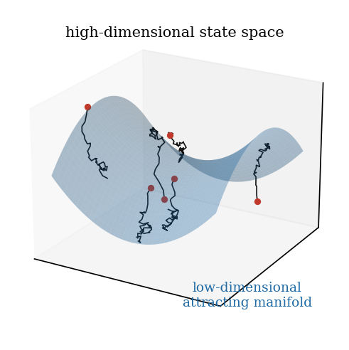
Figure 8.5 Trajectories of a dissipative system, launched from scattered initial conditions in a high-dimensional state space, collapse onto a low-dimensional attracting manifold. Reduced-order models seek coordinates on this manifold.#
The oldest and most widely used of these methods is proper orthogonal decomposition (POD), known in other fields as principal component analysis. Given a collection of snapshots of a field – successive velocity fields of a turbulent flow, say – POD finds the fixed spatial patterns, or modes, ordered so that the first captures as much of the variance (the energy) as possible, the second as much of the remainder, and so on [Berkooz et al., 1993]. For flows with coherent structure, the energy is concentrated in a mere handful of modes, and the field can be reconstructed from them to good accuracy (Figure 8.6). The high-dimensional field is thereby reduced to the evolution of a few modal amplitudes – a small dynamical system of the kind studied in this book.
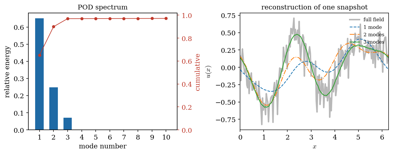
Figure 8.6 Proper orthogonal decomposition of a field with low-dimensional structure. Left: the energy is captured almost entirely by the first three modes. Right: a single snapshot, reconstructed with one, two and three modes, converges rapidly to the full field; the residual is noise.#
POD organises a field by energy, but says nothing about its dynamics. A complementary idea is to seek modes that evolve simply in time. Dynamic mode decomposition (DMD) extracts from a sequence of snapshots the patterns that grow, decay and oscillate at definite rates [Schmid, 2010], and is closely tied to the Koopman viewpoint (Figure 8.7): although the flow \(\dot{\mathbf{x}} = \mathbf{f}(\mathbf{x})\) is nonlinear in the state, it acts linearly on functions of the state, the observables [Mezić, 2005]. In exchange for moving to a higher-dimensional space of observables, one recovers a linear description – with all the eigenvalues and modes that linearity brings – of a nonlinear system.
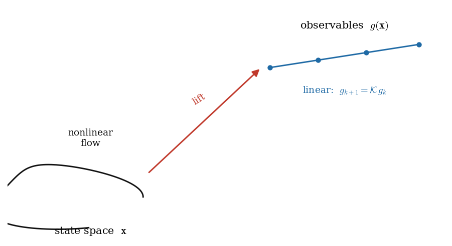
Figure 8.7 The Koopman viewpoint. The flow is nonlinear in the state \(\mathbf{x}\), but by lifting to a space of observables \(g(\mathbf{x})\) it can be represented by a linear operator \(\mathcal{K}\). Dynamic mode decomposition approximates this operator from data.#
POD, DMD and the Koopman operator are best seen not as competing techniques but as three expressions of a single idea: finding low-dimensional structure in a high-dimensional system. It is this idea, rather than any particular algorithm, that endures – and it is a direct descendant of the observation, made throughout this book, that dissipative chaotic systems live on attractors far smaller than their phase space.
The same idea underlies the more recent, and more fashionable, use of machine learning in dynamical systems. It is best regarded not as a replacement for the theory of this book but as one more way to do two familiar things: to approximate the nonlinear operator \(\mathbf{f}\) of (8.1) when it is unknown or too expensive to evaluate, and to discover low-dimensional coordinates for a complex system when the linear modes of POD are not flexible enough. A neural-network surrogate that emulates an expensive model is doing the former; an autoencoder that compresses a high-dimensional field to a few latent variables is doing the latter, and its latent space is simply a nonlinear version of the attracting manifold of Figure 8.5. Presented this way, the methods are variations on the themes of the previous sections rather than a new subject, and we do not dwell on them here; the monograph of Brunton and Kutz [2019] develops the connection between machine learning, dynamical systems and control at length.
8.4. Harnessing chaos#
The chapter so far has treated chaos as an adversary – something to be predicted around, corrected for, or compressed away. Yet the very properties that make a chaotic system hard to predict can also be put to use. Sensitive dependence stretches and folds, which is exactly what is needed to mix; the dense set of unstable orbits buried in an attractor makes it exquisitely controllable; and the way a single variable carries the imprint of the whole attractor lets us reconstruct the dynamics from one measured signal. We take these three in turn.
Stirring milk into coffee mixes it in seconds, but at the small scales of a microfluidic channel the flow is smooth and slow, and molecular diffusion alone would take an age. The way out is that a fluid element's position can behave chaotically even when the flow itself is simple and laminar – this is chaotic advection [Aref, 1984, Aref and Balachandar, 1986]. A convenient model advects each element \((x_n,y_n)\) on the unit square through one period of a time-periodic flow by two successive shears,
with both coordinates taken modulo one so that the fluid stays on the square. This is a close relative of the standard map of chapter 3: each shear merely slides fluid along one direction and so preserves area, as an incompressible flow must, yet for an amplitude \(A\) of order one the map stretches and folds a blob of dye into ever finer filaments (Figure 8.8), until diffusion across the thin lamellae finishes the job. Shaping a real channel so that its flow is chaotic in this way is now a standard route to efficient micromixers for drug delivery and diagnostics, and the same mechanism stirs the mantle, the oceans and the atmosphere.
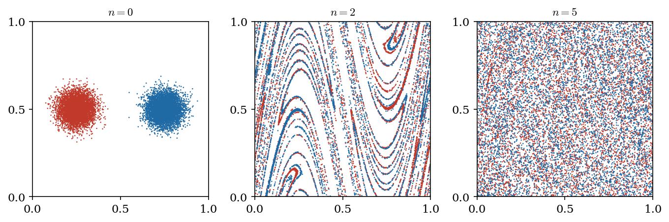
Figure 8.8 Chaotic mixing. Two blobs of dye advected by a simple time-periodic flow are stretched and folded into ever finer filaments and, within a few periods, interleaved throughout the domain – efficient mixing produced by a smooth, laminar flow.#
Maple
The map (8.4) is just the two shears applied in turn; wrap keeps the dye on the unit square by taking each coordinate modulo one. Iterating it on a thin streak of points reproduces the filaments of Figure 8.8.
restart: with(plots):
A := 0.9:  wrap := t -> t - floor(t):          # stay on the unit torus
step := proc(p) local xn:                      # one period of the flow
  xn := wrap(p[1] + A*sin(2*Pi*p[2])):         # horizontal shear
  [xn, wrap(p[2] + A*sin(2*Pi*xn))]:           # vertical shear
end proc:
blob := [seq([0.25, 0.40 + 0.2*k/100], k=0..100)]:   # a thin streak of dye
for n to 5 do blob := map(step, blob): end do:
pointplot(blob, symbol=point, view=[0..1, 0..1]);
Coherent structures and ocean transport
The same template scales up to the planet. In the ocean and atmosphere the stretching and folding organise themselves around hidden curves and surfaces – the Lagrangian coherent structures – that act as the transport barriers and conduits of the flow, the moving skeleton along which tracers are funnelled [Haller, 2015]. Computed from satellite-derived surface currents, they predict where an oil slick will spread or where a person lost at sea will drift; attracting structures were found to coincide with the observed extent of the Deepwater Horizon spill, and the same calculation now guides search-and-rescue operations and the tracking of drifting plastic. The fractal, folded interfaces of chapter 7 and these coherent structures are two views of the one stirred, chaotic flow.
The second use turns sensitivity into control. A chaotic attractor is far from structureless: threaded through it is a dense set of unstable periodic orbits, each a perfectly regular motion that the system shadows briefly before sensitive dependence throws it off. Because the trajectory passes close to any chosen orbit sooner or later, and because sensitive dependence means a tiny nudge has a large effect, one can stabilise that orbit with vanishingly small, well-timed adjustments of a parameter – the method of Ott et al. [1990]. Figure 8.9 demonstrates it on the logistic map \(x_{n+1} = r\,x_n(1-x_n)\) of chapter 2. The target is its unstable fixed point \(x^{*} = 1 - 1/r\), and the control at step \(n\) is the change in growth rate that would send the current state exactly there; solving \((r+\delta r_n)\,x_n(1-x_n) = x^{*}\) gives
applied only while it stays small, \(|\delta r_n| \le \delta r_{\max}\). Because the orbit repeatedly strays near \(x^{*}\), and a per-cent-level nudge is then enough to catch it, the once-chaotic iteration is captured onto the fixed point and held there indefinitely. A regular system would need a large control to be moved so far; it is precisely the chaos that makes such delicate steering possible. The same idea has been used to suppress the arrhythmic beating of cardiac tissue [Garfinkel et al., 1992] and to tame the flickering output of lasers.
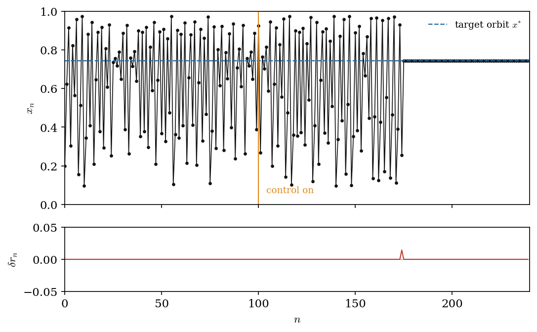
Figure 8.9 Controlling chaos. Left of the marker the logistic map (\(r=3.9\)) iterates chaotically. Once control is enabled it waits until the orbit strays near the target fixed point \(x^{*}\) and then, with the minuscule parameter nudges \(\delta r_n\) shown below, locks the motion onto it.#
Maple
Controlling the logistic map costs only a few lines: at each step, if the state is near the target \(x^{*}\), nudge \(r\) by the small amount (8.5) that would map it exactly onto the fixed point.
restart: with(plots):
r := 3.9:  xstar := 1 - 1/r:  drmax := 0.05:   # target orbit and largest nudge
x := 0.2:  orbit := NULL:
for n to 240 do
  rr := r:
  if n > 100 then                              # switch the controller on
    dr := xstar/(x*(1-x)) - r:                 # nudge that would hit x*
    if abs(dr) <= drmax then rr := r + dr: end if:
  end if:
  x := rr*x*(1-x):
  orbit := orbit, [n, x]:
end do:
plot([orbit], style=point, symbolsize=6);
The third use reads chaos from data. In an experiment one seldom measures the full state; more often a single scalar is recorded – a voltage, a velocity at one point, the interval between drips of the faucet of chapter 3. Remarkably, that lone time series is enough. Takens' theorem [Takens, 1981] guarantees that the vectors built from delayed copies of one coordinate, \((x_t,\, x_{t+\tau},\, x_{t+2\tau},\ldots)\), trace out a faithful copy of the original attractor, with the same dimension, Lyapunov exponents and topology. Figure 8.10 rebuilds the Lorenz attractor from its \(x\)-coordinate alone. This delay embedding is what lets the box-counting and correlation dimensions of chapter 7 be measured from a real signal, and it underpins the analysis of chaotic data across science – detecting the approach of an epileptic seizure from an EEG, diagnosing incipient faults in rotating machinery, and forecasting ecological and physiological records.
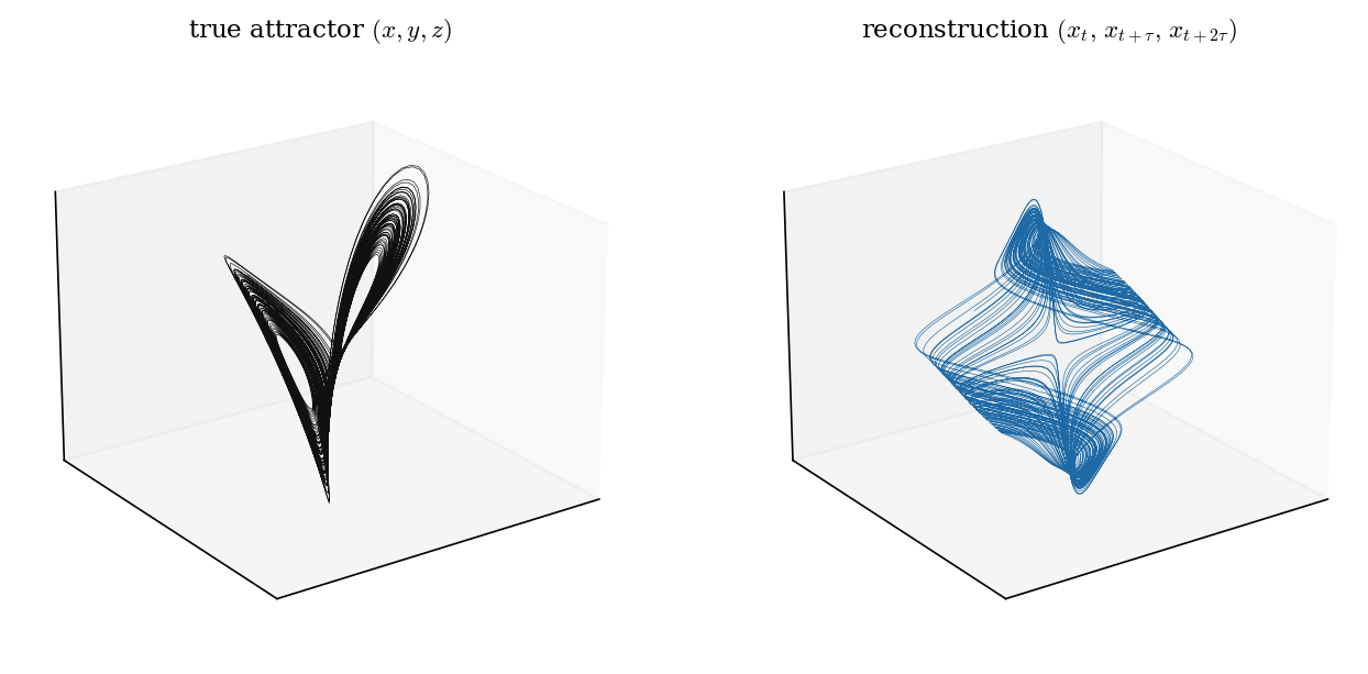
Figure 8.10 Attractor reconstruction. From the single recorded coordinate \(x(t)\) of the Lorenz system (left), the delay-coordinate vectors \((x_t, x_{t+\tau}, x_{t+2\tau})\) trace out a reconstruction (right) with the same two-lobed topology as the original – the content of Takens' theorem.#
Maple
Reconstruction needs only a single recorded coordinate. If the list X holds the sampled values \(x(t_i)\) of a Lorenz run, the delay vectors are formed and plotted directly.
restart: with(plots):
tau := 18:                                     # delay, in samples
N   := nops(X) - 2*tau:
emb := [seq([X[i], X[i+tau], X[i+2*tau]], i=1..N)]:
pointplot3d(emb, symbol=point, symbolsize=1, axes=boxed);
Fingerprinting a chemical reactor
The delay-embedding idea is not confined to the laboratory. Industrial fluidised beds and bubble columns – workhorses of the chemical industry – are strongly nonlinear and, in many operating regimes, chaotic. A single, cheaply measured pressure signal is enough to reconstruct their attractor, and the shape of that attractor, together with a measure of its unpredictability (the Kolmogorov entropy), serves as a fingerprint of the hydrodynamic state (Figure 8.11) [van den Bleek et al., 2002]. The chaotic-processes group at Delft – the very setting from which this book grew, with Floris Takens himself involved – turned this fingerprint into a suite of industrial tools: characterising flow regimes and their transitions, guiding the scale-up of reactors by matching attractors, and even controlling the bubbling. A small, energy-neutral feedback adjustment of the gas supply forces the bed onto a chosen unstable periodic orbit – the control idea of this section applied to a reactor – and was shown to raise the yield of a catalytic reaction by more than ten per cent. The same fingerprint drives an early-warning system: by continuously comparing the live attractor with a healthy reference one, the onset of particle agglomeration is caught long before a conventional pressure-drop alarm would trip, in time to keep the reactor from clogging solid.
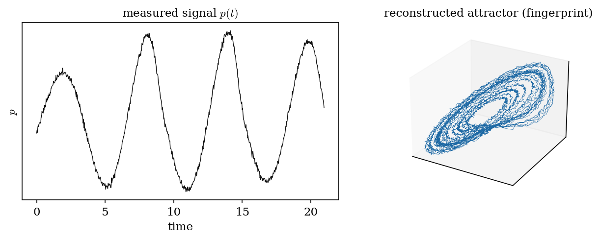
Figure 8.11 The Takens route in industry (illustrative). A single measured signal – here a noisy chaotic time series standing in for the pressure in a fluidised-bed reactor (left) – is turned by delay embedding into a reconstructed attractor (right). The shape of this "fingerprint" characterises the operating regime, and changes in it give early warning of malfunction.#
8.5. Why nonlinear dynamics matters#
The applications sketched here are far from solved problems. Predicting the coupled ocean–atmosphere system across the many scales of climate, closing the equations of turbulence, modelling living systems and steering large engineered networks all remain among the hardest challenges in computational science. What they share is the difficulty this book has been about from the start: they are nonlinear, high-dimensional and sensitive to their initial conditions, so that brute-force prediction fails and one must instead reason about ensembles, attractors and reduced descriptions.
We began by asking how a system as simple as a one-dimensional map or three coupled equations could defeat prediction. In answering it, you have acquired something more general than a catalogue of chaotic phenomena. The finite horizon that forces us to forecast with ensembles, the correction of models by data, the low-dimensional structure hidden inside high-dimensional systems, and the recognition that the same sensitivity can be turned to advantage – to mix, to control, to reconstruct – are not facts about the Lorenz equations; they are habits of thought that apply wherever nonlinear systems are modelled. You have not merely learned about chaos – you have learned to think about nonlinear systems, and that is a tool for the whole of modern science and engineering.
8.6. Exercises#
8.6.1. The predictability horizon#
Consider the Lorenz equations with the standard parameters \(\sigma=10\), \(r=28\), \(b=8/3\).
a) Starting from a point on the attractor, integrate an ensemble of \(M=400\) initial conditions drawn from a small Gaussian blob of width \(\delta_0\). Measure the ensemble spread \(\delta(t)\) and verify that it grows as \(\mathrm{e}^{\Lambda_e t}\) with \(\Lambda_e \approx 0.9\), as in Figure 8.3.
b) Halve the initial spread \(\delta_0\) and repeat. By how much does the predictability horizon increase? Explain, using the relation \(t_{\text{h}} \approx \Lambda_e^{-1}\log(\delta_{\text{att}}/\delta_0)\), why improving the initial condition buys only a logarithmically longer forecast.
c) At what value of \(\delta(t)\) does the exponential growth cease? Relate this saturation level to the size of the attractor.
8.6.2. A Kalman filter for the Lorenz system#
Reproduce the twin experiment of Figure 8.4.
a) Integrate a "truth" trajectory and generate noisy observations of the full state at intervals \(\Delta t_{\text{obs}} = 0.2\), adding Gaussian noise of standard deviation \(1.5\) to each component. Starting from a deliberately wrong initial guess, run a free forecast (no assimilation) and confirm that it diverges from the truth within the predictability horizon.
b) Implement the extended Kalman filter of section 8.2, reusing the Jacobian \(J\) of chapter 6 to propagate the covariance. Show that the analysis tracks the truth and that its RMS error stays well below that of the free forecast.
c) Study the effect of the observation frequency and noise. What happens as \(\Delta t_{\text{obs}}\) is increased towards the predictability horizon? What happens if only the \(x\)-component is observed instead of the full state?
8.6.3. Reduced-order structure#
a) Build a synthetic field \(u(x,t) = \sum_{k=1}^{3} a_k(t)\,\phi_k(x)\) from three fixed spatial patterns \(\phi_k(x)\) whose amplitudes \(a_k(t)\) are the three components of a Lorenz trajectory, and add a little noise. Form the snapshot matrix and compute its singular value decomposition.
b) Plot the singular values. How many modes are needed to capture \(99\%\) of the energy, and how does this relate to the number of patterns you put in?
c) Reconstruct a single snapshot using one, two and three modes and compare with the full field, as in Figure 8.6. What does the part that the leading modes fail to capture correspond to?
8.6.4. Controlling the logistic map#
Consider the logistic map \(x_{n+1} = r\,x_n(1-x_n)\) at \(r=3.9\), where the dynamics are chaotic.
a) Locate the unstable fixed point \(x^{*} = 1 - 1/r\) and confirm, from the derivative of the map, that it is unstable.
b) Implement the OGY idea of section 8.4: at each step, if the state is close enough to \(x^{*}\), choose the small parameter change \(\delta r_n\) that would map \(x_n\) exactly onto \(x^{*}\), applying it only when \(|\delta r_n|\) is below a chosen bound. Show that the orbit is captured onto \(x^{*}\) and held there, as in Figure 8.9.
c) How does the time taken to capture the orbit depend on the size of the allowed perturbation? What happens if the bound is made very small?
8.6.5. Reconstructing an attractor from one signal#
a) Integrate the Lorenz system and keep only the \(x(t)\) time series. Form the delay-coordinate vectors \((x_t, x_{t+\tau}, x_{t+2\tau})\) and plot the reconstructed attractor for a few values of the delay \(\tau\), as in Figure 8.10.
b) Estimate the correlation dimension (section 7.3) of the reconstructed attractor and compare it with the value obtained from the full three-dimensional trajectory. Are they consistent, as Takens' theorem requires?