1. The Maple cookbook#
This Maple cookbook contains various routines or 'recipes' for the analysis of non-linear and chaotic dynamical systems. The aim of this document is to provide you with a set of recipes that will enable you to analyze physical systems quickly and effectively. By no means is this document intended to be a sufficient introduction into Maple, although it should give a reasonable impression of how Maple works and what it can do in this field.
1.1. Settings & tips#
Always use Worksheet mode, never Document mode
Tools \(\rightarrow\) Options \(\rightarrow\) Interface \(\rightarrow\) default format for new worksheets: set to Worksheet
Tools \(\rightarrow\) Options \(\rightarrow\) Display \(\rightarrow\) Input display: set to "Maple Notation"
Tools \(\rightarrow\) Options \(\rightarrow\) General \(\rightarrow\) Auto save: uncheck (i.e. no auto-saving)
1.2. Useful keys#
Ctrl-J: insert execution group after cursor
Ctrl-K: insert execution group before cursor
Ctrl-delete: remove line
F3: split execution group
F4: join execution group
SHIFT-Enter: new line without execution (for loops)
Try them now!
1.3. Help#
Maybe the most important command is the ? command, which is to get help about a certain command.
Maple
? solve
1.5. General#
A session normally starts with a restart command, clearing all data from memory and with including some packages, such as plots for figures and DEtools for differential equations
Maple
restart; with(plots): with(LinearAlgebra): with(DEtools):
Some important details:
All commands need to end with ; or :
: suppresses output from that command.
You can put more than one command on an execution line.
Assigning a value to a variable is done with :=. A common mistake is to use = instead of :=, but = is used for equations, not assignments. Note the crucial difference below:
a = 1/sqrt(2);
a;
note: \(a\) has not been assigned, i.e. \(a\) did not get a value, however a := 1/sqrt(2);
a;
1.6. Floating point numbers#
Maple is a mathematical language and will allways try to give an exact answer. So 1/2 and 0.5 are not the same, and we will need to specifically ask Maple to convert the result to a float: evalf(a);
By Typing Digits;
maple shows you how many digits its uses, which is by default 10. You can control the accuracy by setting Digits to a different number.
Maple
Digits := 60:
evalf(Pi);
1.7. Functions vs expressions#
A function and an expression, respectively, are defined as
Maple
f := x -> x^2;
Maple
q := x^2;
Asking for the value of a function is easier (and more elegant) than for an expression f;
f(2);
Maple
subs(x=2, q);
Note that \(f\) does not evaluate, and that \(f(x)\) is an expression. f; f(x);
Using the unapply command you can convert an expression into a function:
Maple
q := sin(x^2);
Maple
g := unapply(q,x);
Maple
g(y);
The command diff can be used to differentiate functions/expressions
Maple
dg := diff(g(x),x);
Maple
dq := diff(q,x);
Unfortunately, diff does not return a function but an expression. We can cast it into a function with the command unapply:
Maple
dg := unapply(dg,x);
However, the command D returns a function directly.
Maple
dg := D(g);
Maple
dg(z);
We prefer to use functions above expressions in the recipes that follow below.
Functions of more variables are defined very similar, as
Maple
r := (x, y) -> sqrt(x^2 + y^2);
Maple
r(s,t);
Differentiating with respect to \(x\) gives
Maple
diff(r(x,y),x);
The D command can also be used for taking partial derivatives and returning a function:
Maple
drdx := D[1](r);
Maple
drdy := D[2](r);
1.8. Plotting#
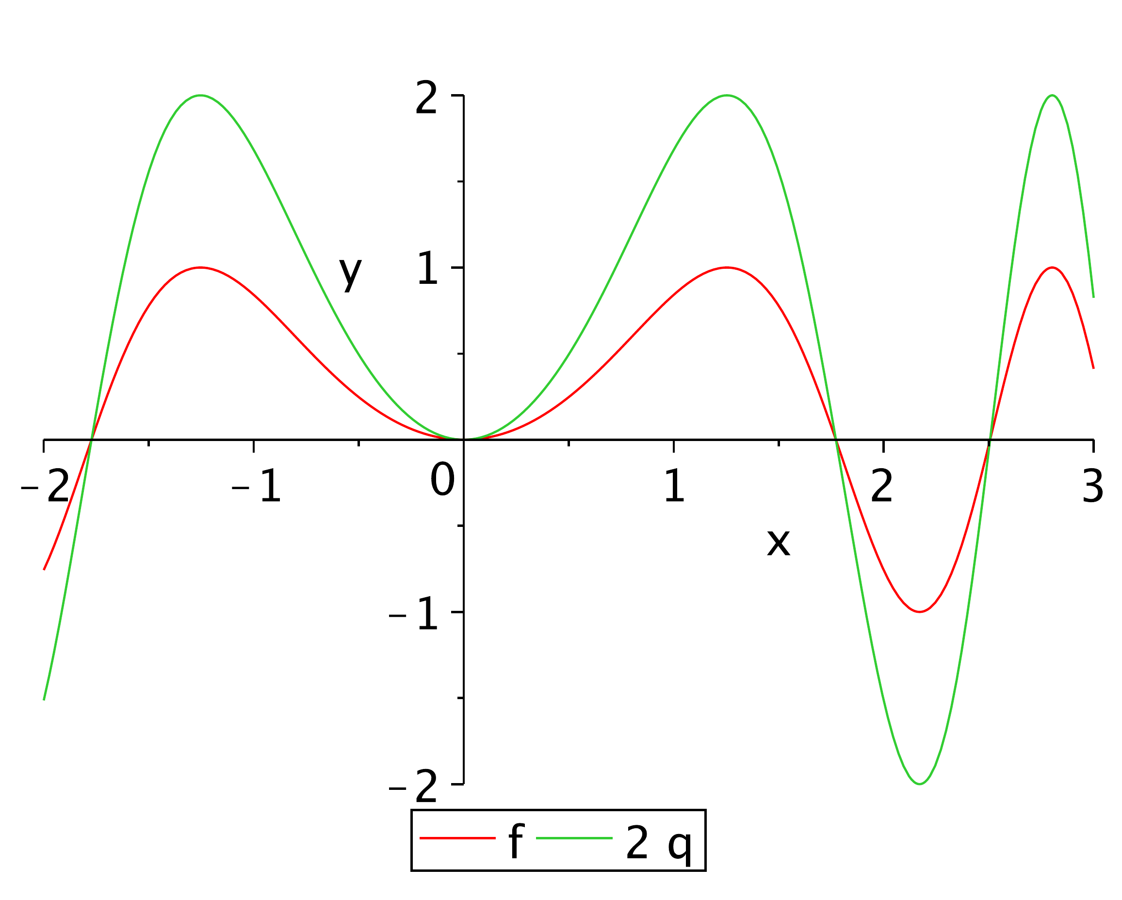
Plotting functions and expressions can be done as follows:
Maple
plot([g(x), 2*q], x=-2..2, labels=["x", "y"], legend=["f","2 q"]);
1.9. Lists, sets, sequences, Arrays, Matrices and Vectors#
A mathematical as well as a programming language, Maple has quite a number of native data types, which can be confusing when starting with Maple. The sequence is one of the most basic data types:
Maple
a := 1,2,3,2,1; b := 1,2,3,4,5; a[3];
An important feature that we will use occasionally is that it is very easy to append elements to sequences. pp := NULL defines pp as an empty sequence.
Maple
c := NULL; # start with an empty sequence
Maple
c := c, 1;
Maple
c := c, 2;
However, the capabilities of sequences are quite limited. For more features, there are the list [ ] and set { } types. Lists can have doubles and preserve order, whereas sets don't. The essential difference between set / lists and sequences is that sets/lists are regarded as one object, whereas sequences aren't.
Maple
seta := { a };
Maple
lista := [ a ];
The seq command can generate new sequences. It is very powerful and we will need it regularly.
Maple
seq(i^2, i=1..5);
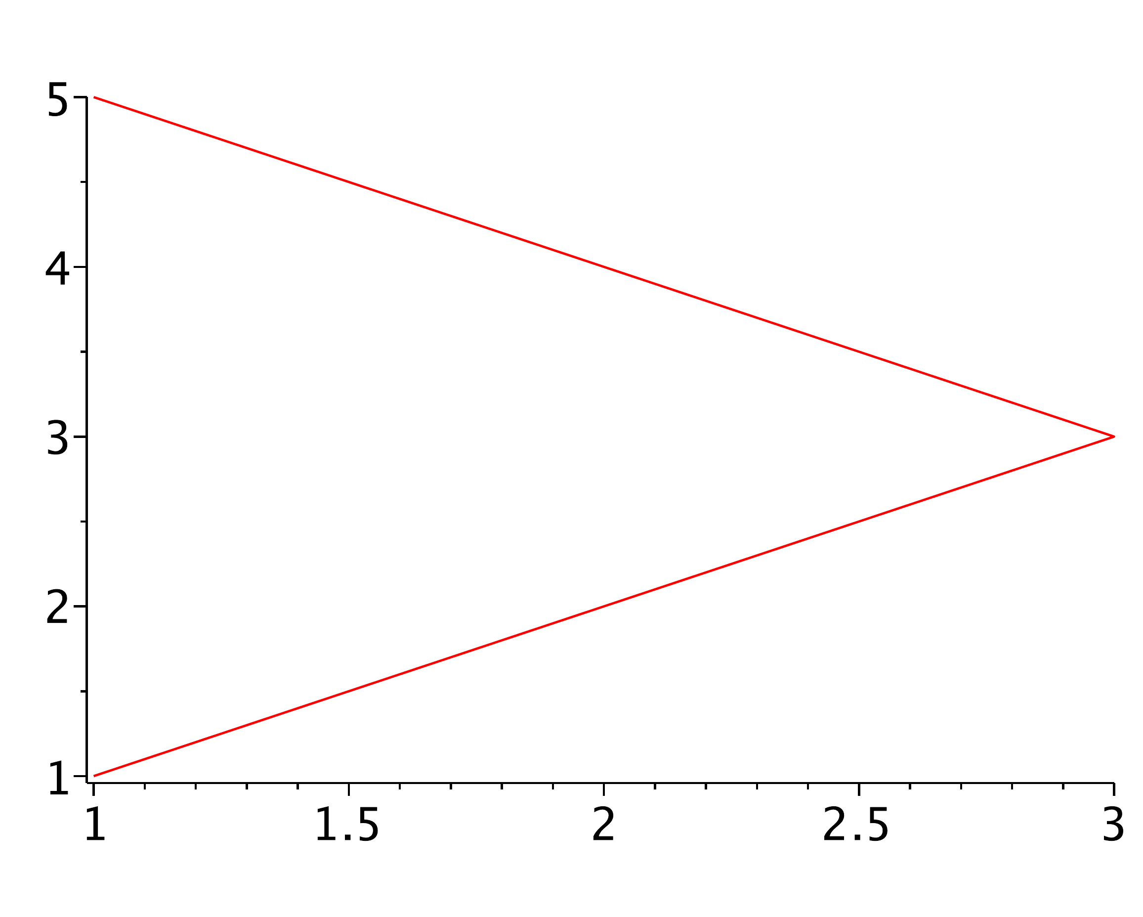
Below we will demonstrate the use of seq to combine the sequences \(a\) and \(b\) into a sequence of list pairs, which can be used to plot the data. Note the detail that plot requires a list (one object) and not a sequence.
Maple
p := seq([a[i], b[i]], i=1..5);
Maple
plot([p]);
To convert a list into a sequence use op, for the number of elements in the list/set use nops.
Maple
lista;
Maple
op(lista);
Maple
nops(lista); # number of elements of lista
Many a time you will want to store data while running through a loop, for example. If you know up front how many elements your data will contain, Arrays are the way to go. Arrays can be declared in various ways, as shown below.
Maple
t := Array(1..10);
Maple
t := Array(1..5,1);
Maple
t := Array([5,3,4,1,2]);
Maple
t := Array(1..5, i -> i);
Maple
t := Array(1..5, i -> i^2);
In the last two examples, an initialization function is used, which uses the index of an Array-element to calculate its value.
Calculating sums & products. Note the following maple oddity with regard to the sum and prod command:
Maple
sum(t[i],i=1..5);
                     Error, bad index into Array
prod(t[i],i=1..5);
                     Error, bad index into Array
Instead use the commands add and mul
Maple
add(t[i],i=1..5);
                               55
mul(t[i],i=1..5);
                             14400
Higher dimensional Arrays are easily created as follows.
Maple
t := Array(1..5, 1..5):
Maple
t := t := Array(1..5, 1..5, (i, j) -> i^2 + j^2);
Matrices and Vectors are basic objects in Maple, and are used as follows:
Maple
A := Matrix([[1,2],[3,4]]);
Maple
b := Vector([1,2]);
Alternatively, you can use a shorthand notation with \(<\), \(>\) and \(|\) symbols. Pay attention that \(|\) indicates a column seperation!
Maple
Aa := <<1,2>|<3,4>>;
Maple
ba := <1,2>;
Note that \(Aa\) is not equal to \(A\)!
Maple
A - Aa;
The functionality of linear algebra is contained in the LinearAlgebra package, which can be included as follows:
Maple
with(LinearAlgebra):
The inverse of A can now simply be found by:
Maple
Ainv := MatrixInverse(A);
Say we want to solve \(A \mathbf{y} = \mathbf{b}\). The vector \(\mathbf{y}\) can now be found by:
Maple
y := Ainv . b;
Which is indeed the solution as verified below.
Maple
b - A . y;
Important: Always type Array, Matrix and Vector with a capital. The types array, matrix and vector exist as well, but are obsolete and work slightly different.
1.10. For-loops#
Frequently we will want to study the behavior of the equations over complete parameter spaces, which can be done with for-loops. These loops are relatively slow, so care needs to be taken when applying them.
Maple
f := x -> sin(x):
N := 25:
X := Array(1..N):
Y := Array(1..N):
for i from 1 to N do
  X[i] := (i-1)*(2*Pi)/(N-1):
  Y[i] := f(X[i]):
od:
X[1..10]; Y[1..10];
For computation speed it may be worthwhile to insert the evalf command
Maple
N := 25:
X := Array(1..N):
Y := Array(1..N):
for i from 1 to N do
  X[i] := evalf((i-1)*(2*Pi)/(N-1)):
  Y[i] := evalf(f(X[i])):
od:
X[1..5];
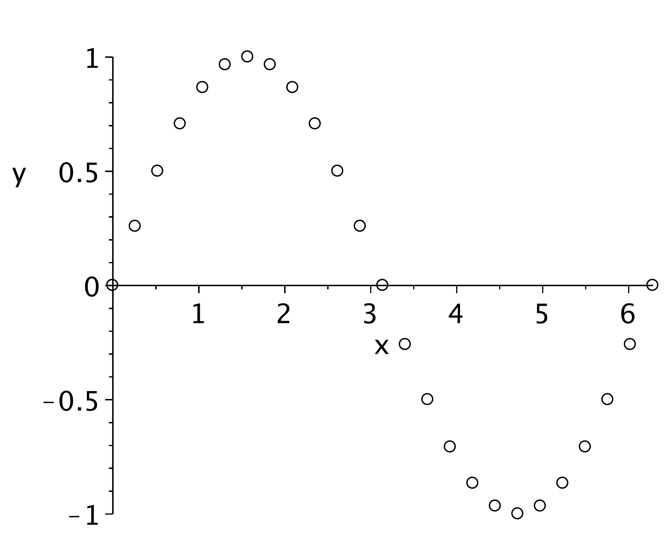
Create a list of \(x,y\) pairs and plot the discrete sine function. The syntax of the plot command for data points is explained below.
Maple
pp := seq([X[i], Y[i]], i=1..N):
plot([pp], style=point,labels=["x","y"],symbolsize=15,symbol=circle);
Occasionally, it may be more convenient to use a list to store our data. This is done as follows:
Maple
N := 25:
pp := NULL:
for i from 1 to N do
  x := (i-1)*(2*Pi)/(N-1):
  pp := pp, [x, f(x)]:
od:
1.11. Plotting data points#
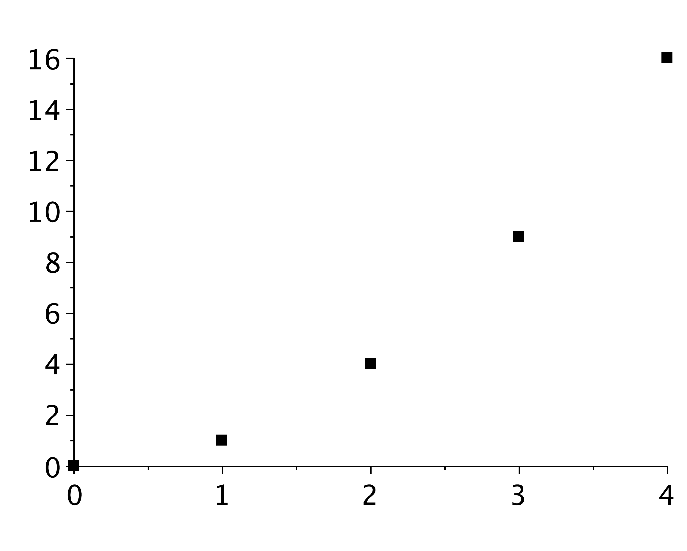
The datatype used for plotting separate datapoints is a list of \(x-y\) pairs: \([ [x_1, y_1], [x_2, y_2] ... ]\). If you specifically want to plot points, use the pointplot command.
Maple
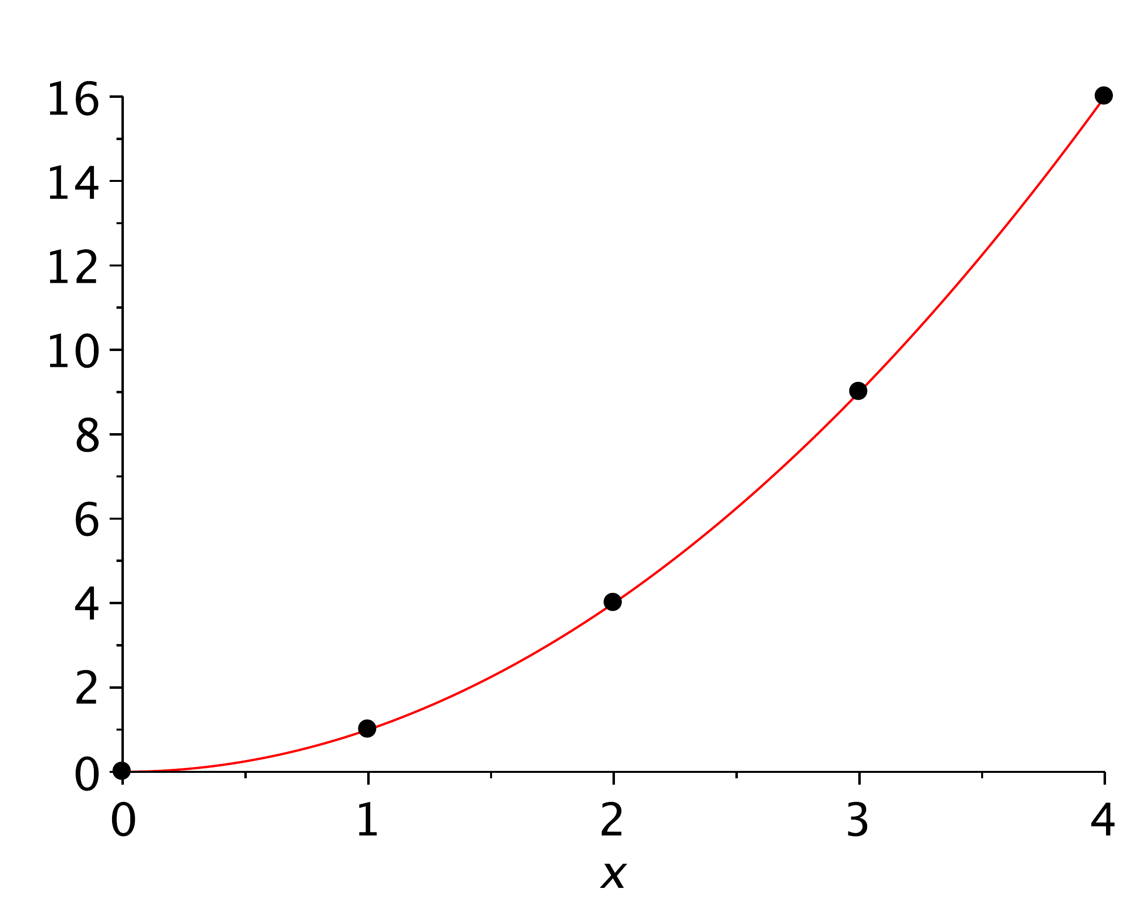
pts := [seq([i, i^2], i=0..4)];
Maple
pointplot(pts,symbolsize=15,symbol=solidbox);
If you also need to plot other functions, plot is the command to use. Note that the variable \(x\) has already been assigned, so we will need to clear it first.
Maple
x := 'x';
plot([x**2, pts], x=0..4, style=[line, point], color=[red, black],
       symbol=solidcircle,symbolsize=15);
1.12. Plotting more than one function at the same time#
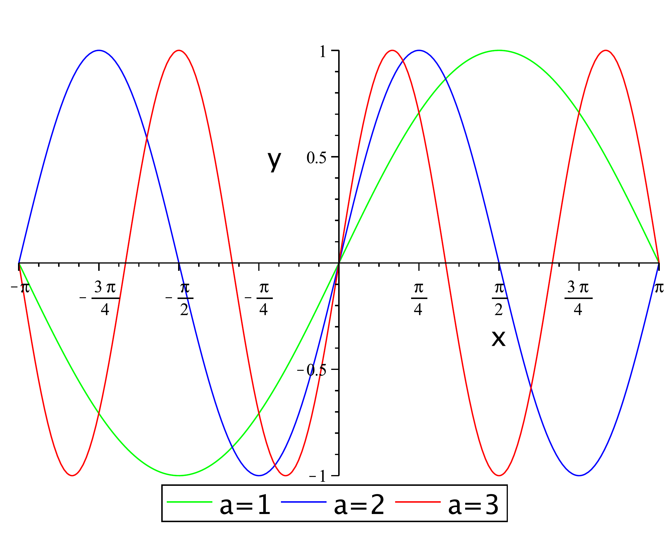
Most of the time, you can simply make a list of expressions that you want to plot:
Maple
restart; with(plots):
f := (x, a) -> sin(a*x);
plot([f(x,1), f(x,2), f(x,3)], x=-Pi..Pi, labels=['x', 'y'],
       legend=["a=1", "a=2", "a=3"], color=[green, blue, red]);
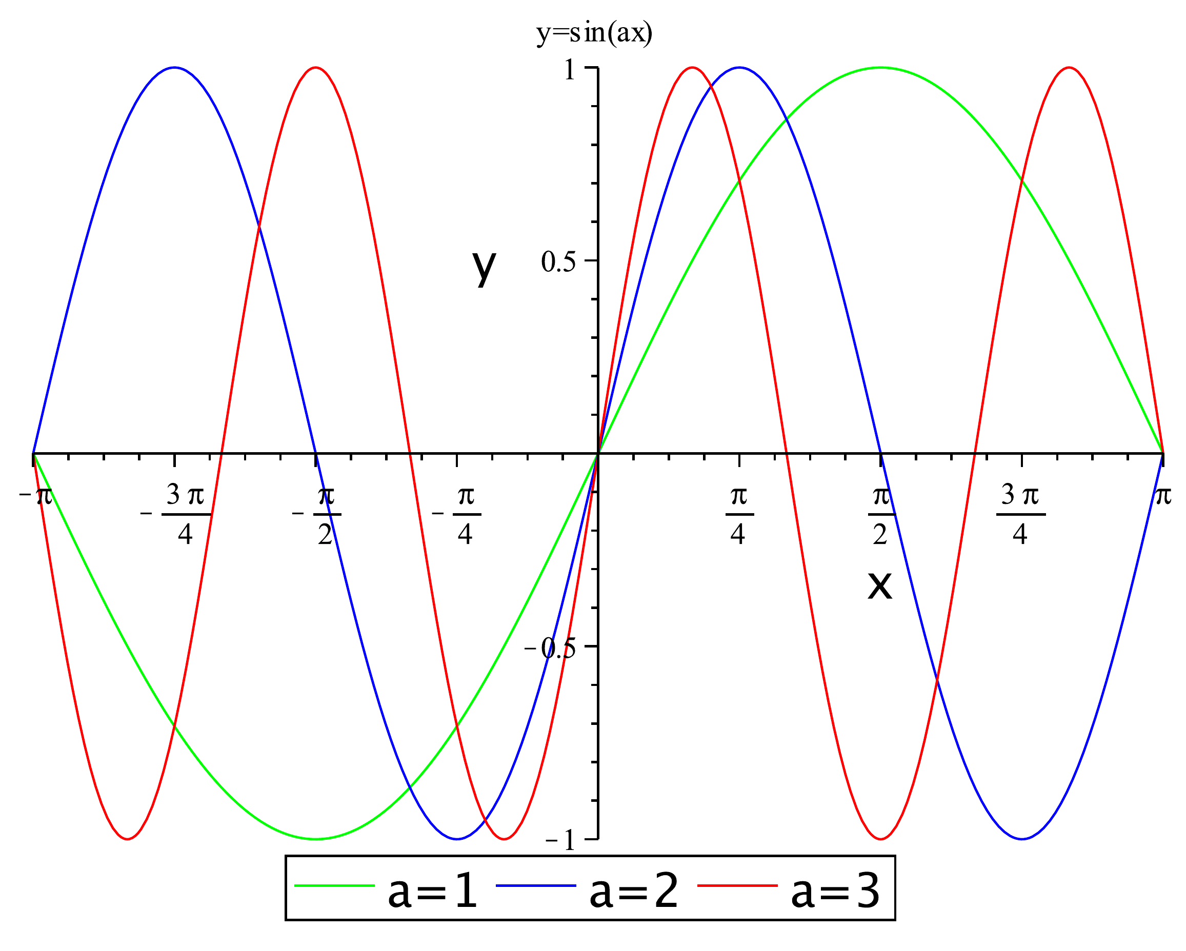
However, sometimes you may want to create the plots separately, and display them on a later moment in one graph. This can be done by using the display command:
Maple
P1 := plot(f(x,1), x=-Pi..Pi, legend="a=1", color=green):
P2 := plot(f(x,2), x=-Pi..Pi, legend="a=2", color=blue):
P3 := plot(f(x,3), x=-Pi..Pi, legend="a=3", color=red):
display(P1,P2,P3,labels=["x","y"]);
1.13. Implicitplot#
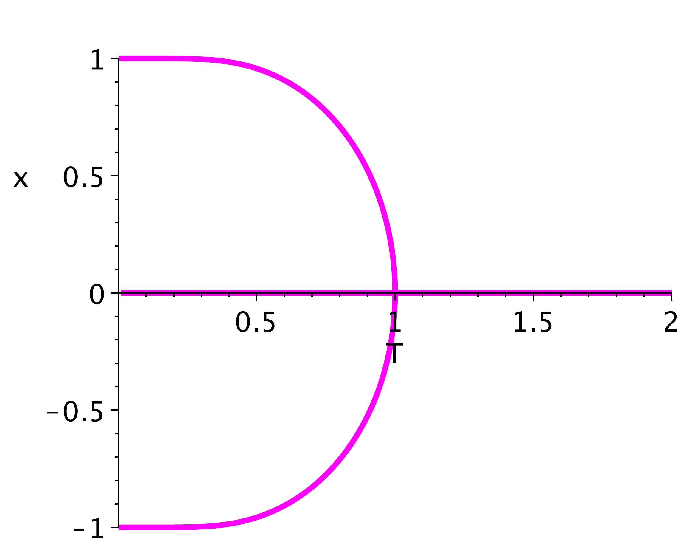
Another very useful is command is implicitplot, which plots implicitly defined data; for example those \(x\) for which \(x=\tanh(x/T)\), as a function of \(T\)
Maple
restart; with(plots):
f := (x, T) -> -x + tanh(x/T):
implicitplot(f(x,T),T=0..2,x=-1.1..1.1,gridrefine=3,labels=["T","x"],
             thickness=4,color=magenta);
1.14. Iterative maps#
Maple
restart; with(plots):
f := x -> r * x * (1 - x);    # define function
N := 50;                      # define nr of points
X := Array(0..N):             # declare data array
r := 0.5;                     # set parameter
X[0] := 0.1;                  # set initial condition
for n from 0 to N-1 do        # perform iterations
  X[n+1] := evalf( f(X[n]) );
end do:
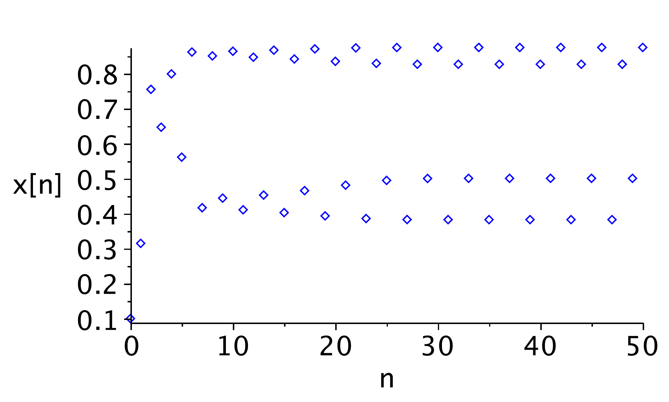
Plot time series (using pointplot)
Maple
l := seq([n,X[n]],n=0..N):
pointplot([l],labels=["n","x[n]"],color=blue,symbol=diamond,symbolsize=12);
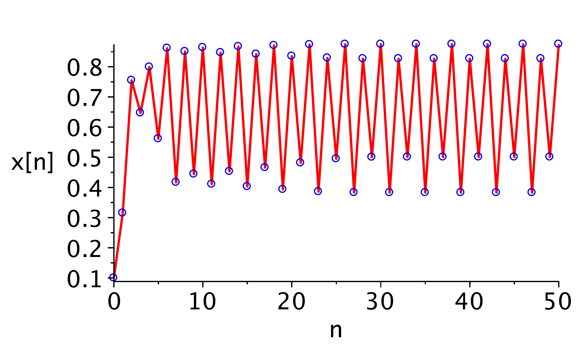
plot time series using more options with plot
Maple
l := seq([n,X[n]],n=0..N):
plot([[l],[l]],labels=["n","x[n]"],color=blue,symbolsize=15,symbol=circle,
       style=[line,point],color=[red,blue],thickness=2);
1.15. Generate cobweb#
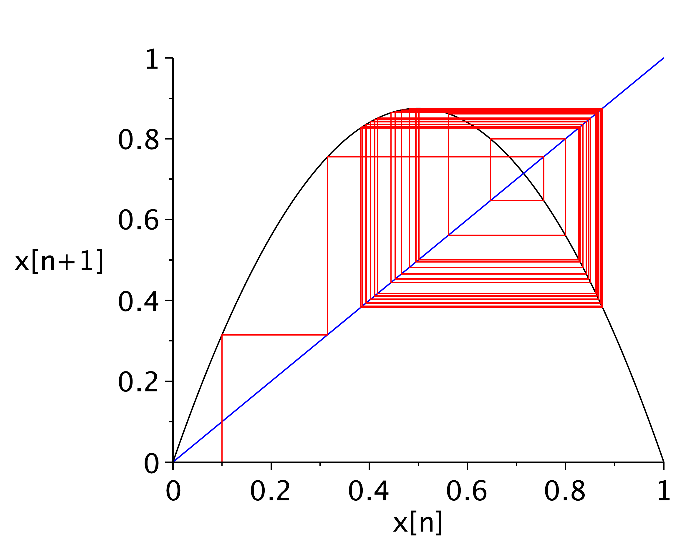
Create and plot a cobweb of the discrete data set
Maple
pp := [X[0], 0]:
for n from 0 to N-1 do
  pp := pp, [X[n], X[n]], [X[n], X[n+1]];
end do:
plot([f(x), x, [pp] ], x=0..1, y=0..1, color = [black, blue, red],
       labels=["x[n]", "x[n+1]"]);
1.16. Return plot#
First we need to create a data series....
Maple
restart; with(plots):
f := x -> r * x * (1 - x);
N := 200:
X := Array(0..N):
X[0] := 0.4: r := 3.8:
for n from 0 to N-1 do
  X[n+1] := evalf(f(X[n]));
end do:
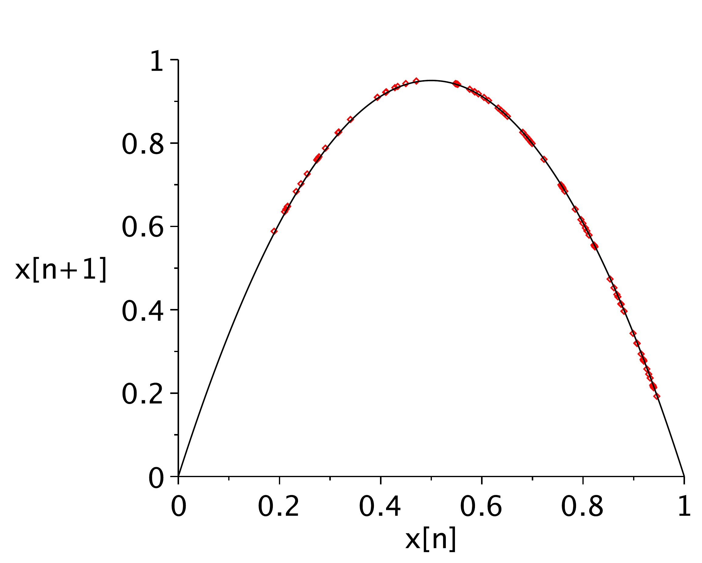
Timeseries X[n] is given. Now create a returnplot by creating [X[n],X[n+1]] pairs and removing the transient by disregarding the first \(N/2\) points
Maple
ret := seq([X[i], X[i+1]], i=N/2..N-1):
plot([[ret], f(x)], x=0..1, 0..1, style=[point, line],color=[red,black],
       labels=["x[n]", "x[n+1]"]);
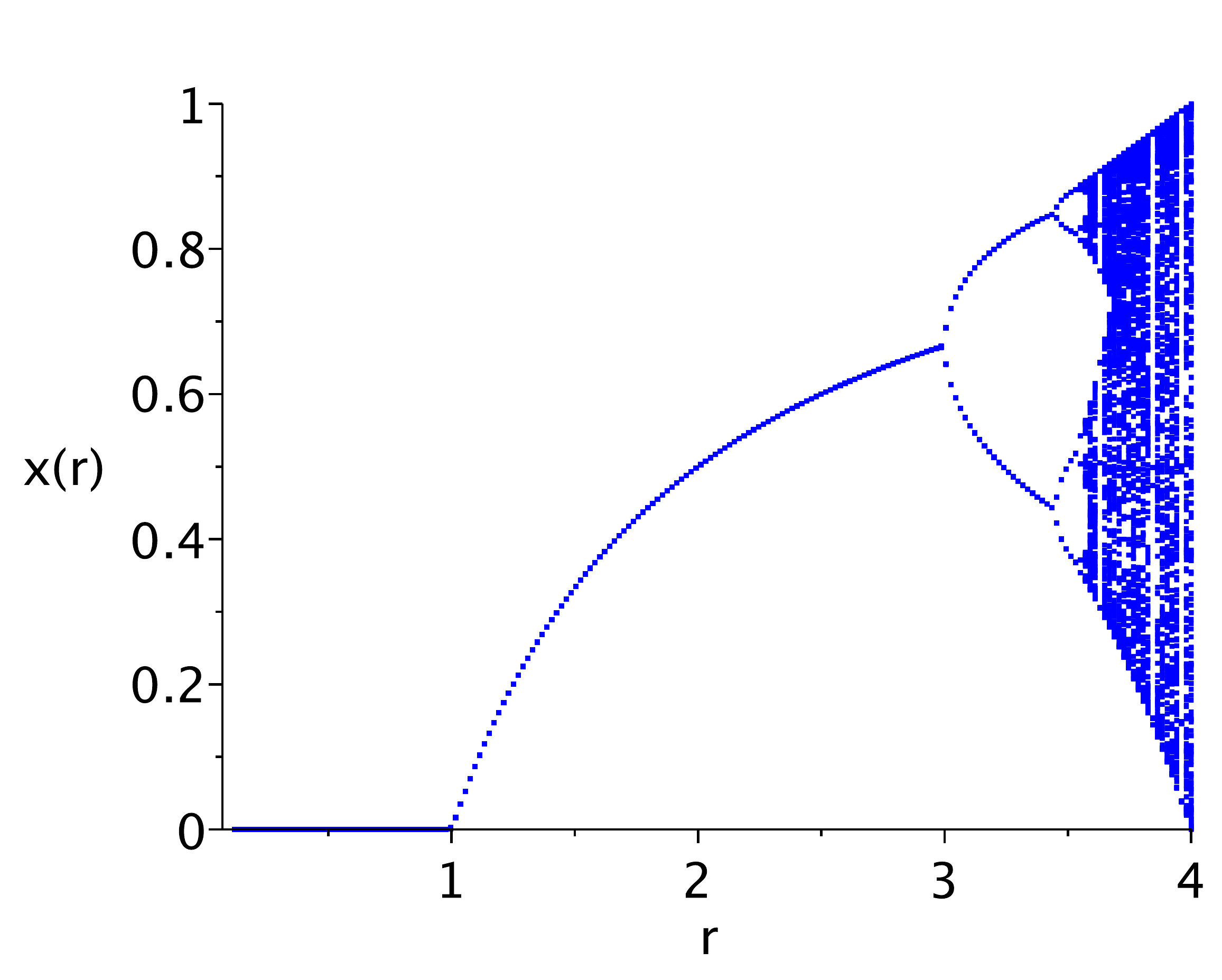
1.17. Bifurcation diagram#
Maple
restart; with(plots):
f := x -> r * x * (1 - x);
N := 500; Nr := 200; rmin := 0.1; rmax := 4;
Nmin := ceil(0.5*N);
X := Array(0..N):
X[0] := 0.57:
for i from 0 to Nr do
  r := evalf(rmin + (rmax - rmin)*i/Nr);
  # Calculate the x[n] series
  for n from 0 to N-1 do X[n+1] := evalf( f(X[n]) ); end do:
  # Store the converged last part as a series for plotting purposes
  pl[i] := seq([r,X[n]],n=Nmin..N);
end do:
# plot the bifurcation diagram
pointplot([seq(pl[i],i=1..Nr)],symbol=POINT,symbolsize=1,
    view=[rmin..rmax,0..1],labels=["r", "x(r)"],color=blue);
1.18. Non-linear differential equations with one variable#
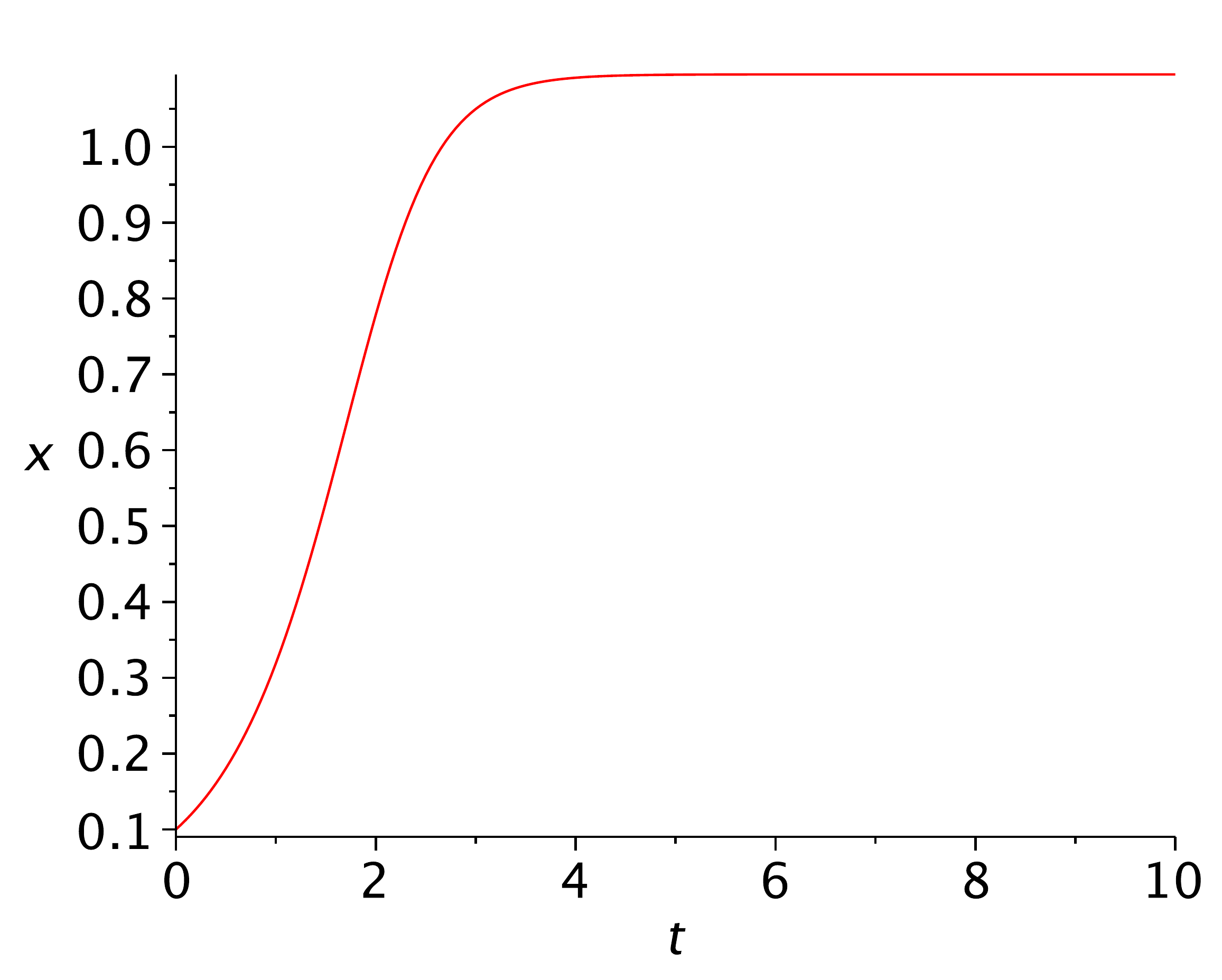
Maple's DEtools package is used for solving differential equations.
Maple
restart; with(plots): with(DEtools):
f := x -> r * x - x^3;
DE := diff(x(t),t) = f(x(t));        # define the differential equation
r := 1.2; x0 := 0.1;                 # set parameter value and initial condition
sol := dsolve({DE, x(0) = x0},x(t),type=numeric); # solve the system numerically
odeplot(sol, [t, x(t)], 0..10);      # plot the numerical approximation
1.19. Bifurcation diagram continuous system#
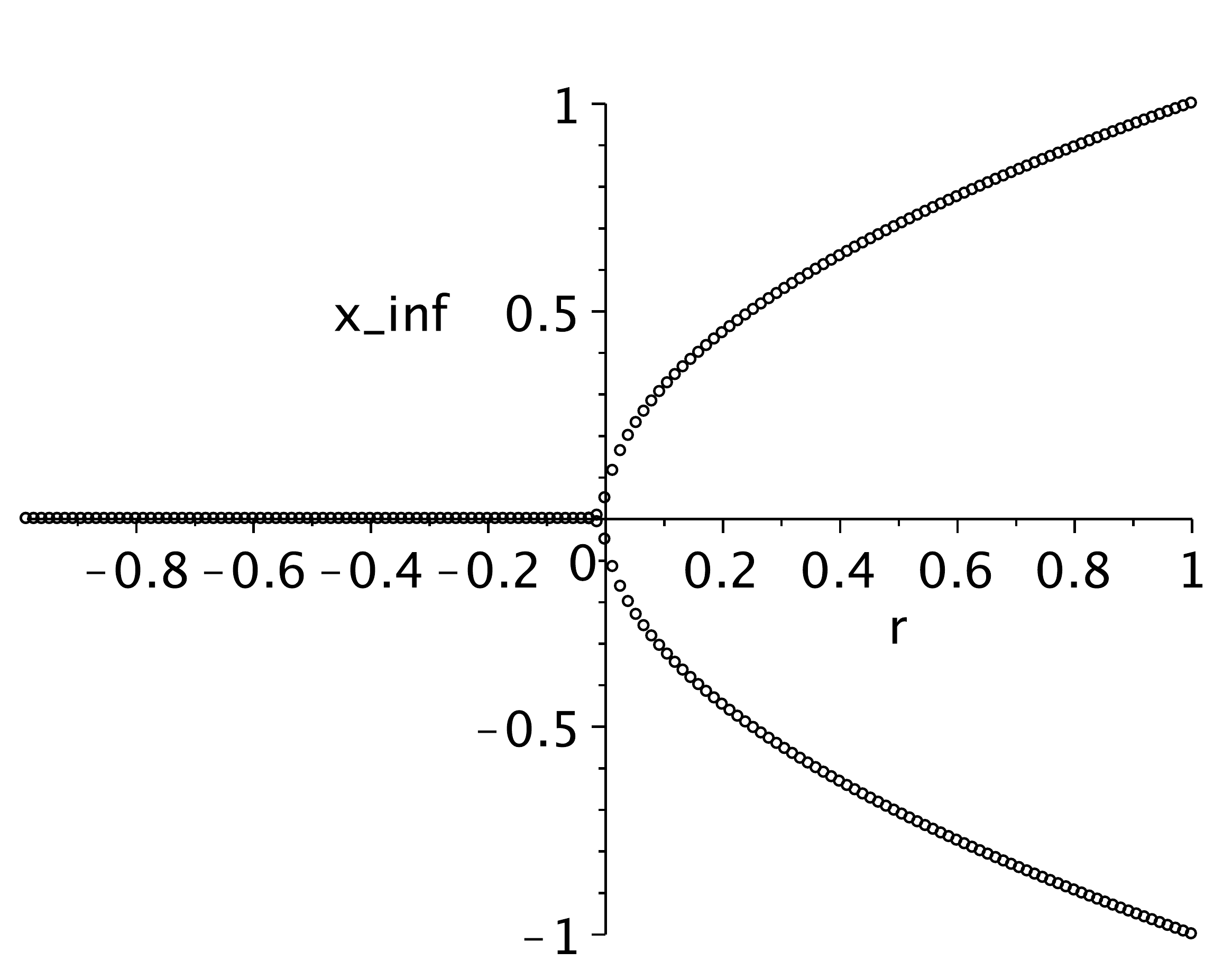
Maple
rmin := -1; rmax := 1; N := 150; tinf := 200;
ic1 := -0.5; ic2 := 0.5;
# calculate the fixed points for various r.

rval  := Array(0..N):
Xinf1 := Array(0..N):
Xinf2 := Array(0..N):
for n from 0 to N do
  r := evalf (rmin + n*(rmax-rmin)/N);

# 'Solve' the DE and evaluate value at tinf

  sol1:=dsolve({DE,x(0) = ic1},x(t),type=numeric):
  sol2:=dsolve({DE,x(0) = ic2},x(t),type=numeric):
  rval[n]  := r;
  Xinf1[n] := subs(sol1(tinf),x(t));
  Xinf2[n] := subs(sol2(tinf),x(t));
od:

# Create a plotlist pp by creating [r, xinf] pairs for both
# initial conditions and plot the results.

pp := seq([rval[n], Xinf1[n]], n=1..N), seq([rval[n],Xinf2[n]], n=1..N):
pointplot([pp], symbol=circle, symbolsize=10, labels=["r","x_inf"]);
1.20. Non-linear differential equations with two dimensions#
We will use an example of the Lotke-Volterra equations of competion.
Maple
restart; with(plots): with(DEtools): with(LinearAlgebra):

f1 := (x, y) -> x * (3 - x- 2 * y);
f2 := (x, y) -> y * (2 - x - y);
DE1 := diff(x(t), t) = f1(x(t),y(t));
DE2 := diff(y(t), t) = f2(x(t),y(t));
DE  := DE1, DE2:
Calculate the fixed points
Maple
sol := solve({f1(x,y)=0, f2(x,y)=0}, {x,y});
For the stability we need to calculate the Jacobian. This can be done using a function from the VectorCalculus package without actually loading the entire VectorCalculus package (you don't want that)
Maple
J := VectorCalculus:-Jacobian([f1(x,y), f2(x,y)], [x,y]);
The Jacobian evaluated at the fourth fixed point is
Maple
J4 := subs(sol[4], J);
Eigenvalues(J4);
Maple
evalf(%);
So the fixed point is a saddle node as \(\lambda_1>0\) and \(\lambda_2 < 0\).
1.20.1. Phase portrait#
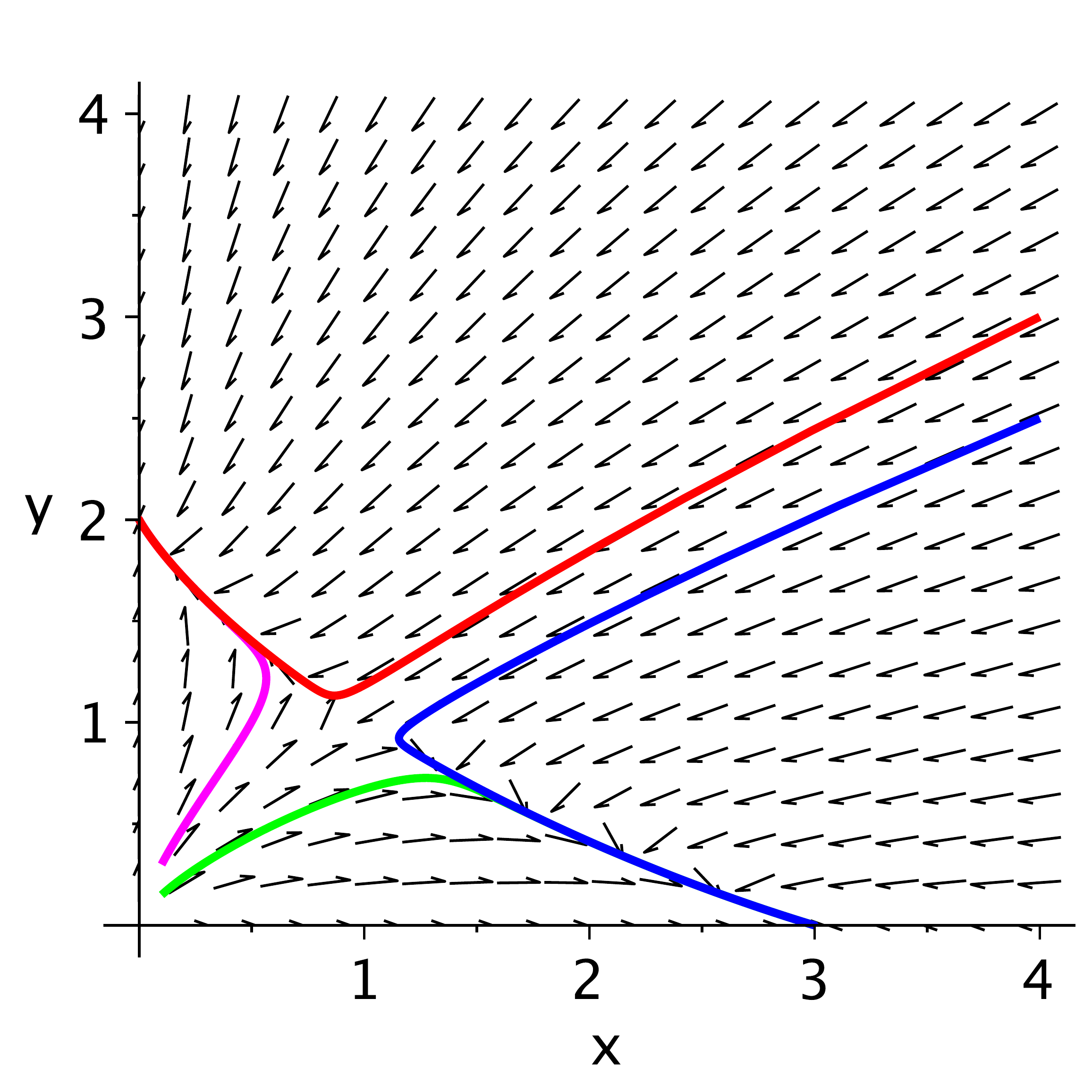
A phase-portrait of the system can be made with the command phaseportrait. In the example the trajectories of four different initial conditions are shown
Maple
phaseportrait([DE], [x(t),y(t)], t=0..50, [[x(0)=0.1,y(0)=0.15],
# x(0)=0.1,y(0)=0.3], [x(0)=4,y(0)=2.5], [x(0)=4, y(0)=3]],
stepsize=0.05, x=0..4, y=0..4, color=black,
linecolor=[green, magenta, blue,red]);
1.21. Non-linear differential equations with three dimensions: chaos#
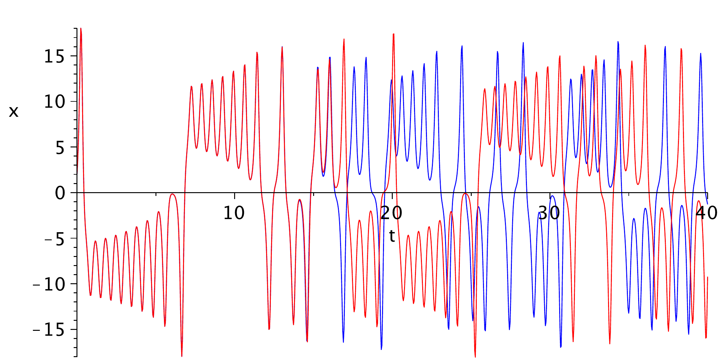
We will use the Lorenz equations as an example
Maple
restart; with(plots): with(DEtools):
# define functions
f1 := (x,y,z) -> sigma * (y - x);
f2 := (x,y,z) -> -x * z + r * x - y;
f3 := (x,y,z) ->  x * y - b * z;
# define differential equations
DE1 := diff(x(t),t) = f1(x(t),y(t),z(t)):
DE2 := diff(y(t),t) = f2(x(t),y(t),z(t)):
DE3 := diff(z(t),t) = f3(x(t),y(t),z(t));
DE := DE1, DE2, DE3;
# define parameters
r:=28; b:=8/3; sigma:=10;
# define two initial conditions close to each other
ic1 := x(0)=2,     y(0)=5,z(0)=5;
ic2 := x(0)=2.0001,y(0)=5,z(0)=5;
# Solve system with dsolve. The option maxfun=-1 allows maple to go beyond
# the default 30,000 function evaluations.
# To see more options we refer to the help.

sol1 := dsolve({DE,ic1},[x(t),y(t),z(t)],type=numeric,maxfun=-1);
sol2 := dsolve({DE,ic2},[x(t),y(t),z(t)],type=numeric,maxfun=-1);

# and plot the timeseries.

p1 := odeplot(sol1,[t,x(t)],0..40,labels=["t","x"],
              numpoints=1000,color=blue,axes=normal):
p2 := odeplot(sol2,[t,x(t)],0..40,labels=["t","x"],
              numpoints=1000,color=red,axes=normal):
display([p1,p2]);
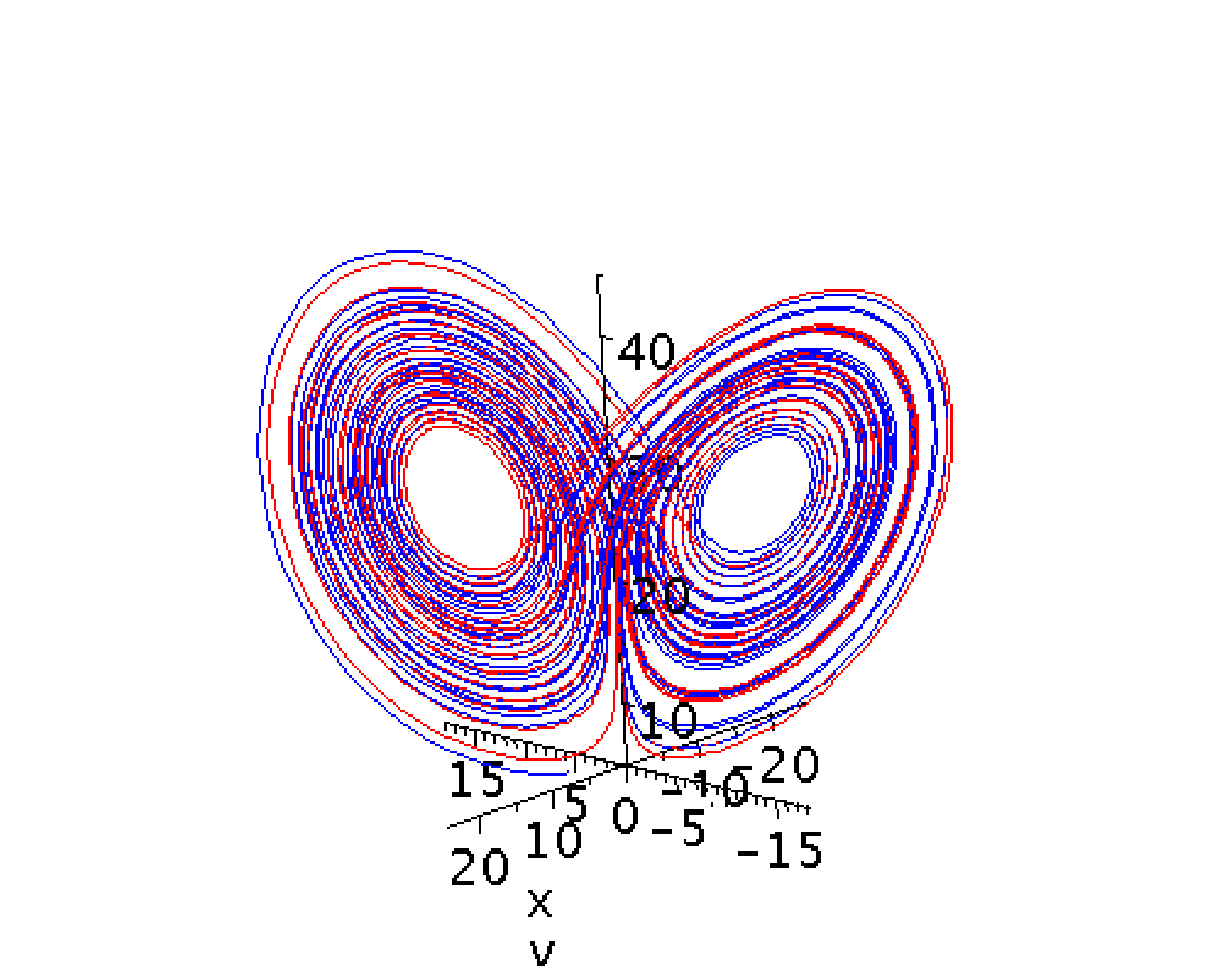
A phase-space plot is created by
Maple
p1 := odeplot(sol1,[x(t),y(t),z(t)],0..40,labels=["x","y","z"],
numpoints=1000,color=blue,axes=normal,numpoints=5000):
p2 := odeplot(sol2,[x(t),y(t),z(t)],0..40,labels=["x","y","z"],
numpoints=1000,color=red,axes=normal,numpoints=5000):
display([p1,p2]);
1.22. Manipulating solutions from dsolve#
Often one would like to be able to manipulate the data obtained from dsolve. This can be done requiring that the numerical data be put into an Array. First create an array which specifies when the data must be sampled.
Maple
N:=2500; dt := 0.01;
samples := Array(1..N, i -(i-1)*dt):
sol_arr := dsolve({DE,ic1},[x(t),y(t),z(t)],type=numeric,maxfun=-1,output=samples):

# The returned data is an Array of Arrays.

sol_arr;
As can be seen, the data is in the second column, with \(t,x,y,z\) respectively. Type "? dsolve/numeric" for more information on dsolve's array format.
Maple
soldd:=sol_arr[2,1];
T := soldd[1..N, 1]:
X := soldd[1..N, 2]:
Y := soldd[1..N, 3]:
Z := soldd[1..N, 4]:
Make a 3D-plot of the Lorenz attractor.
Maple
l3d := seq([X[i], Y[i], Z[i]], i=1..N):
pointplot3d([l3d], axes=boxed, connect = true, labels=["x", "y", "z"]);
1.23. Fractals#
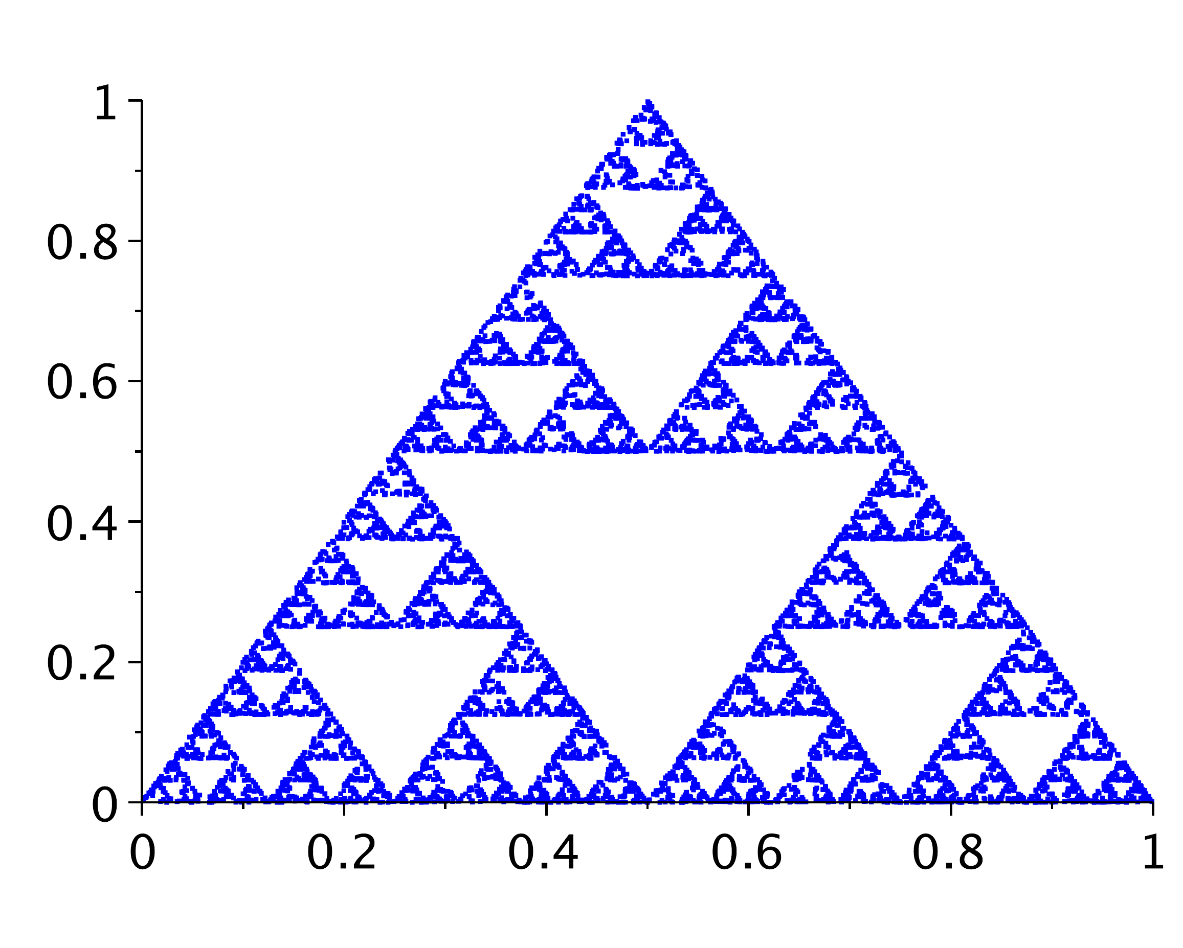
First we have to generate a fractal object. We will do this with a discrete mapping (a chaos game) whose attractor is the Sierpinski gasket, the triangular fractal of dimension \(\log 3/\log 2\) met in the fractals chapter.
Maple
restart; with(plots):
N:=10000;

# Define a random integer generator r for numbers [0,1,2]

r := rand(3):

# Create a X,Y series

X := Array(0..N):
Y := Array(0..N):
X[0] := 1; Y[0] := 0;
for n from 0 to N-1 do

  dice := r();

#  Depending on the result of the dice [0, 1, 2] jump to a new point

  if( dice = 0) then
    X[n+1] := 0.5 * X[n];
    Y[n+1] := 0.5 * Y[n];
  else
    if( dice = 1 ) then
       X[n+1] := 0.5 * X[n] + 0.25;
       Y[n+1] := 0.5 * Y[n] + 0.50;
    else
       X[n+1] := 0.5 * X[n] + 0.5;
       Y[n+1] := 0.5 * Y[n];
    end if;
  end if;
od:

# Create x,y pairs for plot

pp := seq([X[n], Y[n]], n=1..N):
pointplot([pp], symbol=POINT, symbolsize=1, color=blue);
1.24. Calculation box-dimension#
Determine the extrema of the data
Maple
xmin := min(seq(X[i],i=1..N));
xmax := max(seq(X[i],i=1..N));
ymin := min(seq(Y[i],i=1..N));
ymax := max(seq(Y[i],i=1..N));

# Set maximum box-size  and minimum box-size

lmax := max(xmax-xmin,ymax-ymin);
lmin := lmax/100;

# set the number of different box-sizes in the analysis, pmax
pmax := 20;

# the box-size l[p] will vary according to l[p]= lmin*b^p,
# where b is such that l[pmax] = lmax
# calculate b:
b := exp(log(lmax/lmin)/pmax);

# Loop over all resolutions
boxsize := Array(0..pmax):
boxcount := Array(0..pmax):
p := 'p':
print("p, gridsize, boxsize");
for p from pmax to 0 by -1 do
#  Calculate box-size
  boxsize[p] := evalf(lmin*b^p);
#  Calculate the grid-size (ie nr of boxes)
  gridsize := trunc(lmax/boxsize[p])+1;
  print(p,gridsize,boxsize[p]);
# Construct the grid and set the initial values to zero
  grid := Array(1..gridsize, 1..gridsize, 0);

# Mark which boxes in the grid are occupied
  for n from 1 to N do
    i := trunc((X[n]-xmin)/boxsize[p])+1;
    j := trunc((Y[n]-ymin)/boxsize[p])+1;
    grid[i,j] := 1;
  od:

# Count number of occupied boxes
  boxcount[p] := 0;
  for i from 1 to gridsize do
    for j from 1 to gridsize do
       boxcount[p] := boxcount[p] + grid[i,j];
    od;
  od;

od:

# Plot the results in log-log fashion ...

li := seq([log(boxsize[p]),log(boxcount[p])],p=0..pmax):
plot([[li],[li]],style=[point, line],symbolsize=15,color=[blue,red],
     symbol=circle, labels=["log(boxsize)", "log(boxcount)"]);
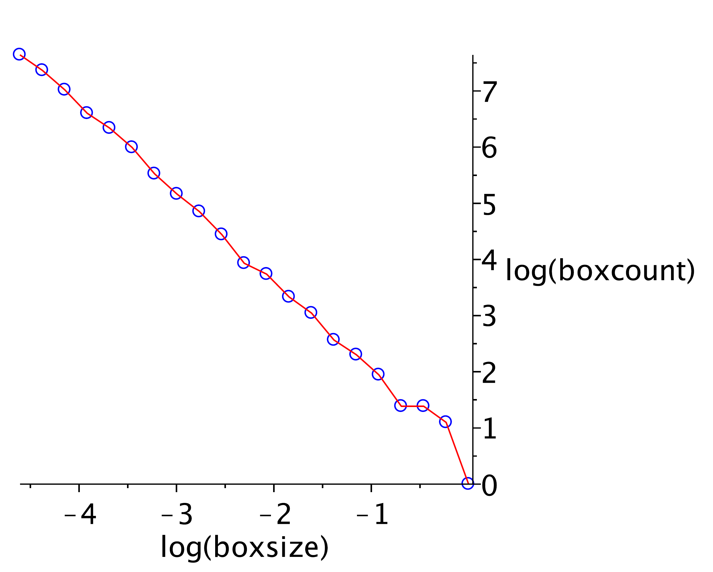
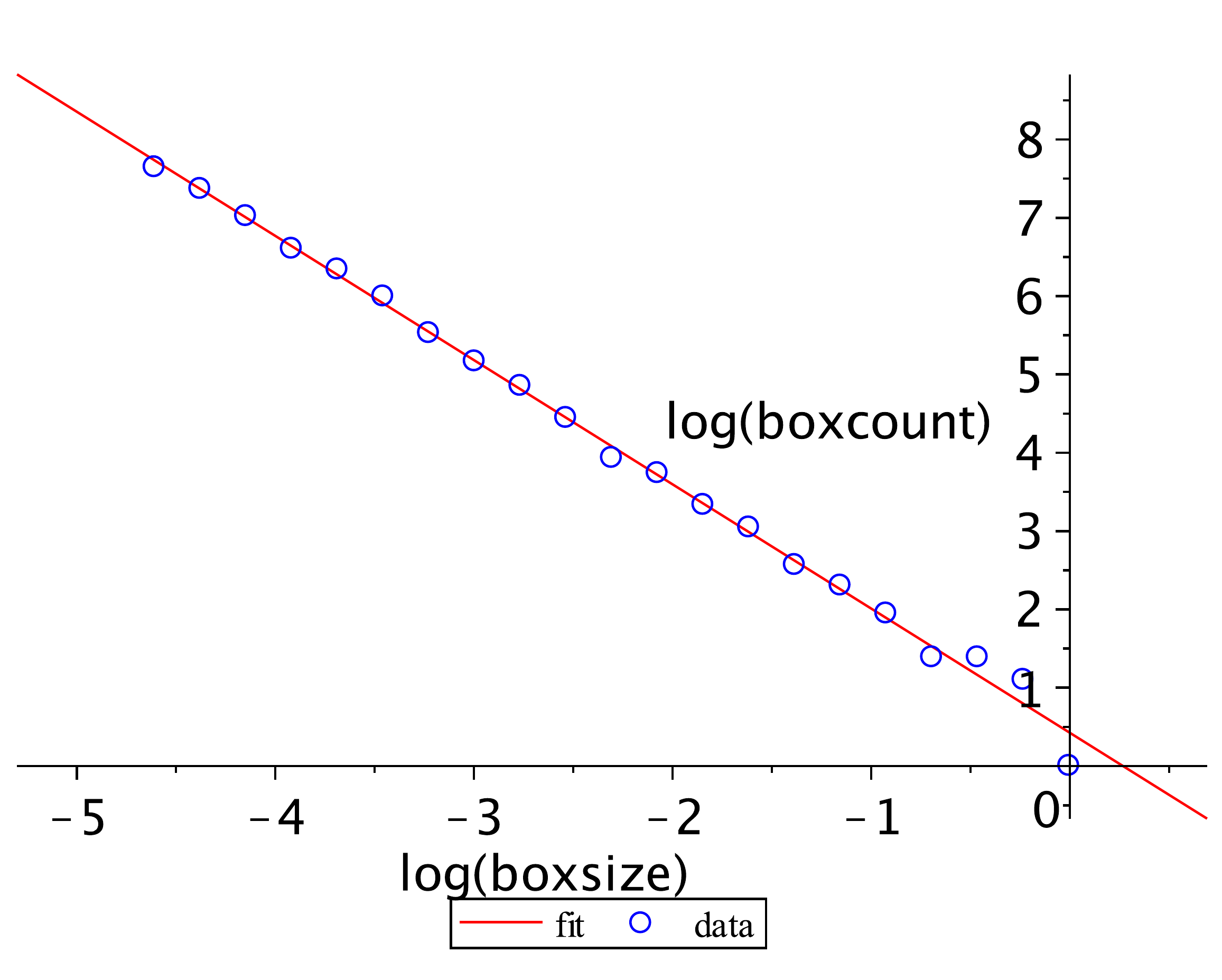
Calculate the box dimension. We could do this by fitting a line using the Fit function from the Statistics package. This fit procedure from the module "Statistics" needs input values in Vector format.
Maple
with(Statistics):
X := Vector([seq(log(boxsize[p]),p=0..pmax)]):
Y := Vector([seq(log(boxcount[p]),p=0..pmax)]):
a := 'a'; b := 'b';
Fit(a + b*x, X,Y, x);
Maple
fit := unapply(%,x);
Maple
plot([fit(x), [li]], x=log(lmin/2)..log(lmax*2), style=[line, point],
     color=[red,blue], symbolsize=15,symbol=circle,
     labels=["log(boxsize)","log(boxcount)"],legend=["fit","data"]);
1.4. Comments#
Maple