1. A start at the end

1.1. Sensitive dependence on initial conditions: the butterfly effect

Around 1960 Edward Lorenz made an odd discovery. Working at MIT Lorenz worked on the issue of weather prediction, but rather than studying the full equations describing atmospheric flow and weather phenomena, he chose to focus on a highly simplified set of equations that still retained some essential elements of the atmospheric system. The governing equations of his abstract system are

(1.1)\[\begin{split}\dot{x} &= \sigma(y-x)\\ \dot{y} &= rx - y -xz\\ \dot{z} &= xy-bz\end{split}\]

where \(r, b\) and \(\sigma\) are parameters and \(\dot{x}\) denotes \(\mathrm{d}x/\mathrm{d}t\). Making use of an early supercomputer he could numerically integrate the equations in time to obtain long-term predictions. In order to be able to calculate the system's behaviour over very long periods, Lorenz sometimes started a new simulation from the 'halfway' result of a calculation that was still running. But when he plotted such a continued calculation together with the original calculation in one graph, he noted to his utter surprise that after a brief period the two curves started to diverge rapidly, ultimately displaying entirely different behaviour. Lorenz figured out that the "stored" values that he used as initial conditions for the second calculations differed slightly from the original values due to round-off effects. This led him to conclude that a minute perturbation of the initial conditions can lead to enormous differences over time. The perspective of weather prediction provided an excellent metaphor to express the effect that small causes can have big impacts: Does the flap of a butterfly's wings in Brazil set off a tornado in Texas?

With a modern PC we can today easily retrace Lorenz' footsteps and experience ourselves the remarkably rich behaviour of his simple system as well as the sensitive dependence on initial conditions. To this end, we start maple and load the file LorenzSensitiveDependence_start.mws, which contains an implementation of the system (1.1), listed below (text comments are preceded by an '[')

Maple

restart; with(plots): with(DEtools):
#  Define the Lorenz equations
f1 := (x, y, z) -> sigma * (y - x);
f2 := (x, y, z) -> -x * z + r * x - y;
f3 := (x, y, z) -> x * y - b * z;
DE1 := diff(x(t), t) = f1(x(t), y(t), z(t)):
DE2 := diff(y(t), t) = f2(x(t), y(t), z(t)):
DE3 := diff(z(t), t) = f3(x(t), y(t), z(t));
DE := DE1, DE2, DE3;
#  Set the parameters
r:=28; b:=8/3; sigma:=10;
#  Set the initial conditions
ic1 := x(0)=2, y(0)=5, z(0)=5;
#  Solve system with dsolve.
sol1 := dsolve({DE, ic1}, [x(t), y(t), z(t)], type=numeric,maxfun=-1);
#  Set the integration range ..
tstart := 0; tend := 30;
#  And plot the timeseries ..
odeplot(sol1, [t, x(t)], tstart..tend, labels=["t","x"]);

Running the entire worksheet produces the time series of \(x(t)\) shown in Figure 1.1.

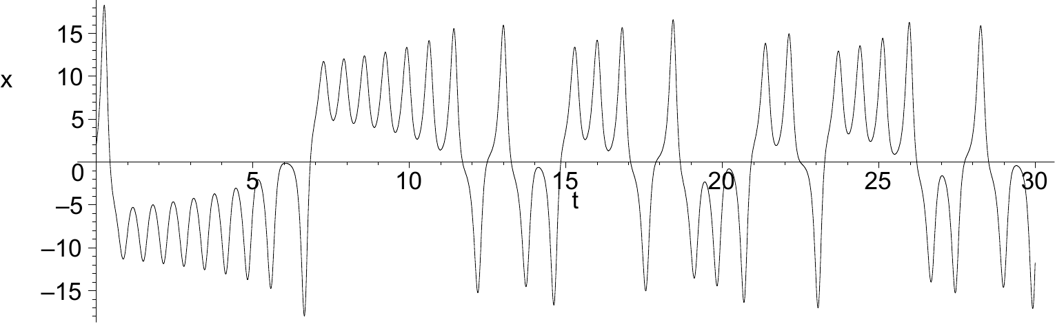
Figure 1.1 Time series \(x(t)\) of the Lorenz system (1.1).

The time series of \(x(t)\) seems to oscillate peacefully, yet no regular pattern has established itself in the range \(t \in [0,30]\). One might suspect that this is merely the transient phase — the period before the system settles into an equilibrium behaviour — and extend the integration time by adjusting tstart and tend to, for example, \(100 \ldots 130\) or \(1000 \ldots 1030\); plotting \(y(t)\) or \(z(t)\) instead of \(x(t)\) tells the same story. However long the integration time is chosen, no regular pattern emerges. This is not yet a proof of chaos, since the transient might simply be even longer. As will be elaborated in the chapters to follow, chaotic behaviour is defined in terms of how sensitively the system responds to a small change in the initial conditions. We can probe this by integrating the Lorenz system for two slightly differing initial conditions: removing the # symbols at the end of the worksheet activates the commands below, which produce plots like Figure 1.2.

Maple

ic2 := x(0)=2+epsilon,y(0)=5,z(0)=5;
epsilon := 1E-3;
sol2 := dsolve({DE,ic2},[x(t),y(t),z(t)],type=numeric,maxfun=-1);
#  plot 2 timeseries in one plot.
tstart := 0; tend := 30;
p1 := odeplot(sol1,[t,x(t)],tstart..tend,labels=["t","x"],color=blue):
p2 := odeplot(sol2,[t,x(t)],tstart..tend,labels=["t","x"],color=red):
display([p1,p2]);

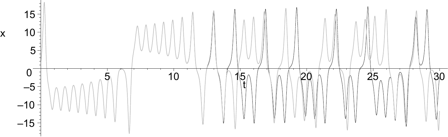
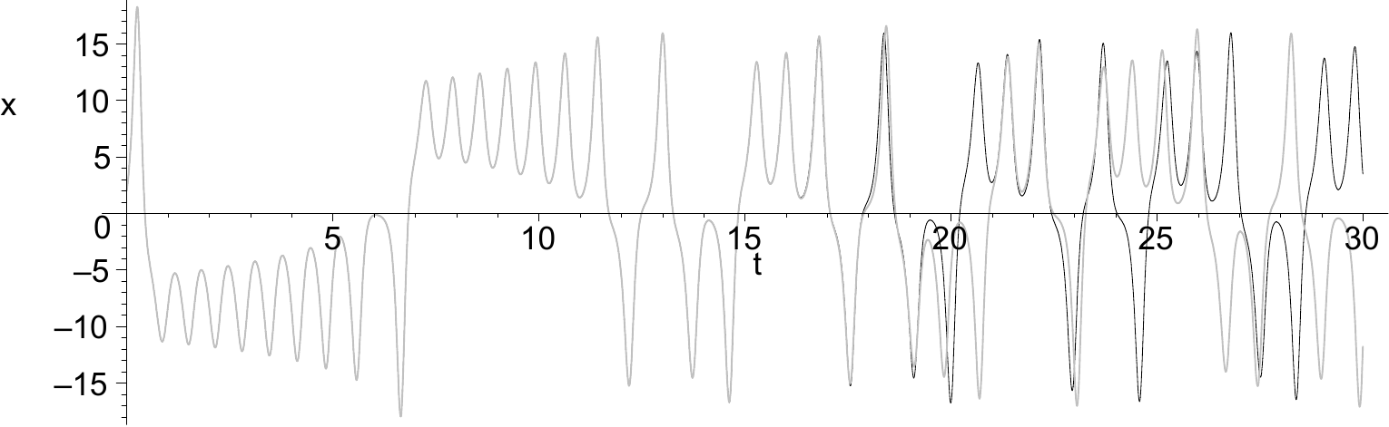
Figure 1.2 Sensitive dependence on initial conditions in the Lorenz-system. Two time-series with slightly differing initial conditions in \(x\): \(x(0)=2\) and \(x(0)=2+\epsilon\), respectively. In all cases \(y(0)=5,z(0)=5\). (a) \(\epsilon = 10^{-3}\). (b) \(\epsilon = 10^{-5}\).

Reducing \(\epsilon\) delays the moment at which the two series visibly diverge, but they always do so eventually. If \(\epsilon\) is made small enough the solutions appear to stay together indefinitely; this is deceptive, however, and reflects the finite accuracy of the computation rather than the dynamics of the system. Increasing the working precision — for instance with > Digits := 20;, which instructs maple to use \(20\) digits instead of the default \(10\) — restores the divergence.

Apart from analysing the time-series, much can be learned by studying the system in the 3d-phase-space. In maple this requires only a minor change of the plot command: odeplot(sol1,[x(t),y(t),z(t)],tstart..tend,labels=["x","y","z"]); which gives a plot like Figure 1.3.

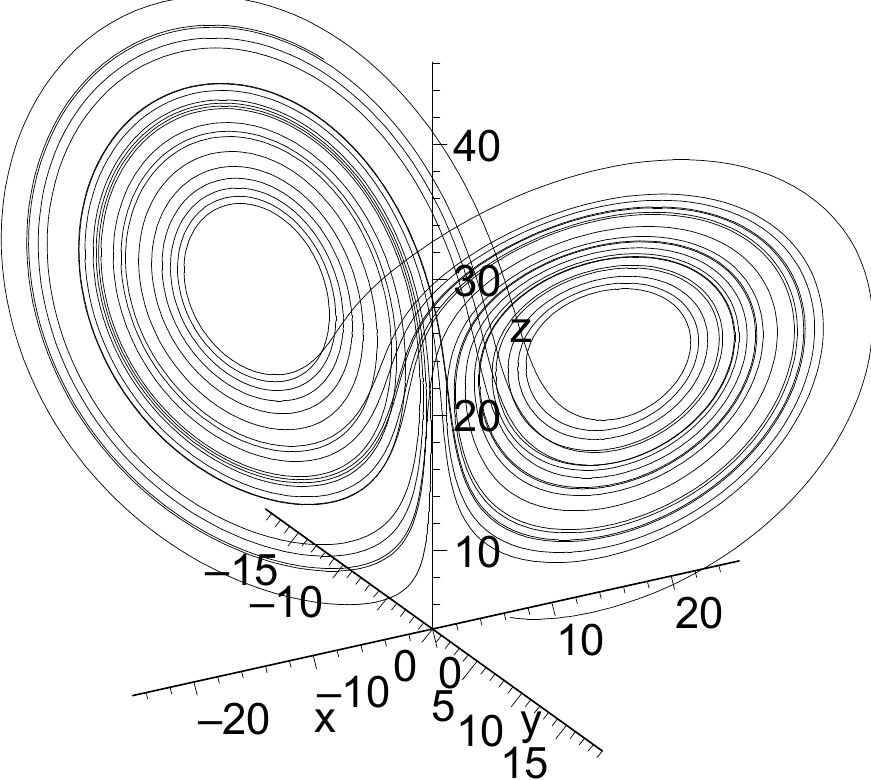
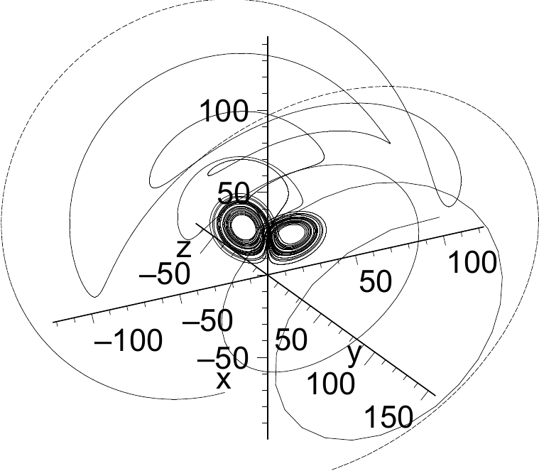
Figure 1.3 Trajectories in phase-space. (a) 'butterfly'-shaped appearance of the system dynamics in phase space. (b) 'attractor'; as the trajectories converge on the butterfly, the object appears to attract the trajectories.

Viewed from various angles, the phase-space trajectory reveals the celebrated butterfly shape. Trajectories launched from different initial conditions — even one as far away as \(x(0) = 100\) — are all drawn onto the same object: they converge upon the attractor (compare Figure 1.3).

See the file LorenzSensitiveDependence.mws for a worked-out maple-sheet. The Lorenz system will be studied in more detail in chapter 6.

1.2. Celestial Uncertainties

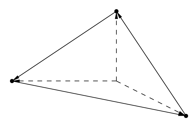
Figure 1.4 Three-body problem.

Imagine three celestial objects – like stars, planets, moons, meteorites and/or satellites – which influence each other by their gravitational pull. Would it be possible to fully predict the future trajectories of these three interacting objects?

It may come as a surprise that the answer turns out to be 'no, not in general'. As discussed during the first lecture, this so-called 'three body problem' has a long history involving among others Euler, Laplace and Poincaré. In the end it was Henri Poincaré who managed to prove that the system cannot be solved analytically in general situations. Only in a few special cases can the solution be expressed in a closed form. To get a feeling for the enormous complexity of the three body problem, we will analyse the system below and calculate numerically some possible trajectories with the aid of maple .

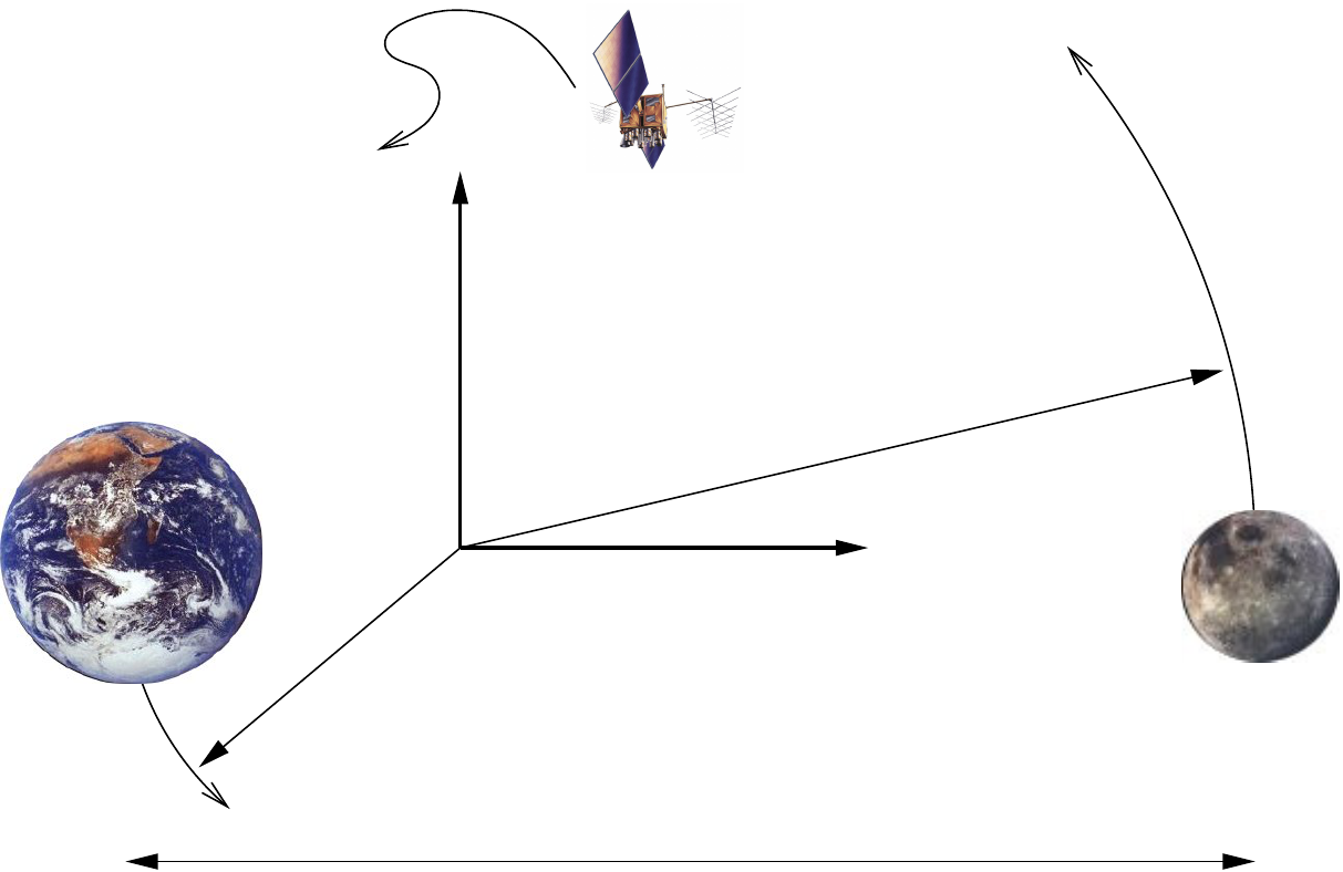
Consider Figure 1.4. The magnitude of the gravitational force of \(m_2\) on \(m_1\) is given by Newton's law

\[ f_{21} = G \frac{m_1 m_2}{\left|\mathbf{x}_2 - \mathbf{x}_1\right|^2} \]

with \(G\) the gravitational constant given in Table 1.1. The direction of this force can be expressed by \((\mathbf{x}_2 - \mathbf{x}_1)/{\left|\mathbf{x}_2 - \mathbf{x}_1\right|}\). Hence the complete three body problem can be written as

(1.2)\[\begin{split}\begin{aligned} m_1 \ddot{\mathbf{x}}_1 &= G m_1 m_2 \frac{\mathbf{x}_2 - \mathbf{x}_1} {\left|\mathbf{x}_2 - \mathbf{x}_1\right|^3} \,\,+\,\, G m_1 m_3 \frac{\mathbf{x}_3 - \mathbf{x}_1} {\left|\mathbf{x}_3 - \mathbf{x}_1\right|^3}\\ m_2 \ddot{\mathbf{x}}_2 &= G m_2 m_1 \frac{\mathbf{x}_1 - \mathbf{x}_2} {\left|\mathbf{x}_1 - \mathbf{x}_2\right|^3} \,\,+\,\, G m_2 m_3 \frac{\mathbf{x}_3 - \mathbf{x}_2} {\left|\mathbf{x}_3 - \mathbf{x}_2\right|^3}\\ m_3 \ddot{\mathbf{x}}_3 &= G m_3 m_1 \frac{\mathbf{x}_1 - \mathbf{x}_3} {\left|\mathbf{x}_1 - \mathbf{x}_3\right|^3} \,\,+\,\, G m_3 m_2 \frac{\mathbf{x}_2 - \mathbf{x}_3} {\left|\mathbf{x}_2 - \mathbf{x}_3\right|^3} \end{aligned}\end{split}\]

The system constitutes a phase-space with dimension 18: three variables each with six degrees of freedom (three-dimensional position and velocity).

This eighteen-dimensional problem can be reduced dramatically by exploiting the particular structure of the earth–moon–satellite setting. Because the satellite (\(m_3\)) is exceedingly light compared with the earth (\(m_1\)) and the moon (\(m_2\)), i.e. \(m_3 \ll m_1,m_2\), it is pulled around by the two heavy bodies but exerts no appreciable influence on them. If, in addition, the two heavy bodies (the primaries) are taken to move on circular orbits about their common centre of mass, and the satellite is confined to that orbital plane, the eighteen dimensions collapse to just four. This reduction, from Newton's law (1.2) to the compact system below, is carried out step by step in Appendix 1. Writing the satellite position as \(\mathbf{x}_{3}(t) = (x(t),y(t))\) and its velocity components as \(u=\dot{x}\), \(v=\dot{y}\), the resulting equations of motion are

(1.3)\[\begin{split}\dot{x} &= u\\ \dot{y} &= v\\ \dot{u} &= G m_1 [x_1 - x]/d_{1}^{3} \,\,+\,\, G m_2 [x_2 - x]/d_{2}^{3}\\ \dot{v} &= G m_1 [y_1 - y]/d_{1}^{3} \,\,+\,\, G m_2 [y_2 - y]/d_{2}^{3}\end{split}\]

with \(d_1\) and \(d_2\) the distances from the satellite to the earth and to the moon,

(1.4)\[d_1 = \sqrt{(x_1 - x)^2 + (y_1 - y)^2}\,\,\,\,\,\,\,\,\,\, d_2 = \sqrt{(x_2 - x)^2 + (y_2 - y)^2}\]

and the earth- and moon-positions moving on their circular orbits

(1.5)\[\begin{split}\begin{gathered} \left[ \begin{array}{c} x_1 \\ y_1 \end{array} \right]= -\frac{m_2 R}{m_1+m_2} \left[ \begin{array}{c} \cos \omega t \\ \sin \omega t \end{array} \right],\,\,\,\,\,\,\, \left[ \begin{array}{c} x_2 \\ y_2 \end{array} \right]= \frac{m_1 R}{m_1+m_2} \left[ \begin{array}{c} \cos \omega t \\ \sin \omega t \end{array} \right] \end{gathered}\end{split}\]

Here \(R\) is the (constant) earth–moon distance and \(\omega\) the angular frequency of the circular orbit. The parameter values for the problem are listed in Table 1.1. Based on these values one finds for the angular frequency \(\omega = 2.96\cdot10^{-6}\) rad s \(^{-1}\).

Table 1.1 Parameters in the three-body problem.

gravitational constant	\(G\)	\(6.67 \cdot 10^{-11}\)	Nm\(^2\) kg\(^{-1}\)
distance between earth and moon	\(R\)	\(3.84 \cdot 10^{8}\)	m
mass of earth	\(m_1\)	\(5.97 \cdot 10^{24}\)	kg
mass of 'moon' in example	\(m_2\)	\(m_1/4\)	kg
real mass of the moon		\(7.36 \cdot 10^{22}\)	kg

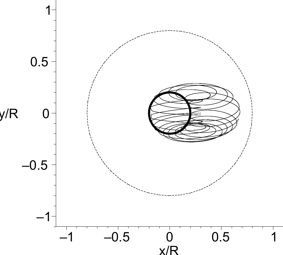
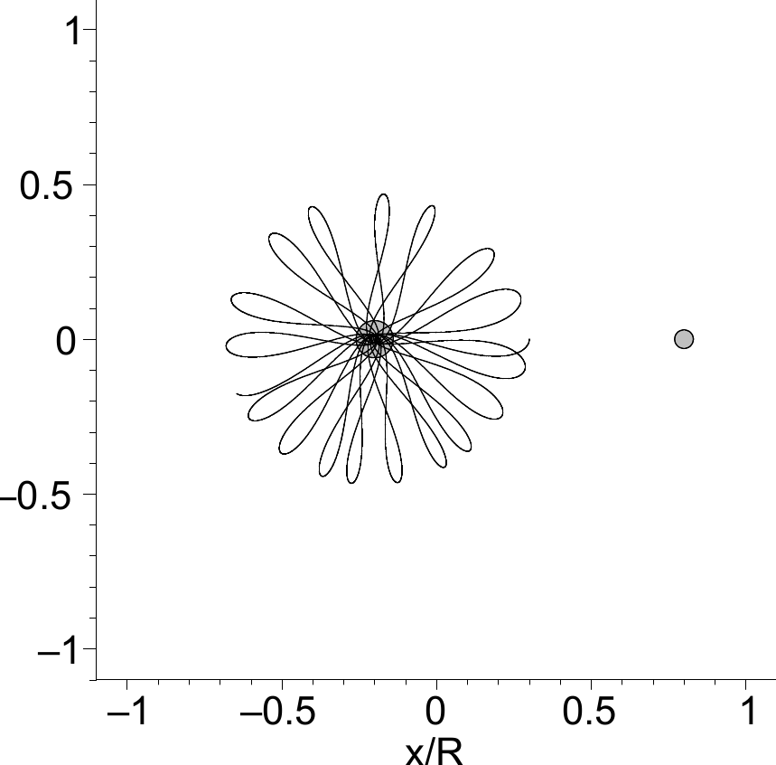
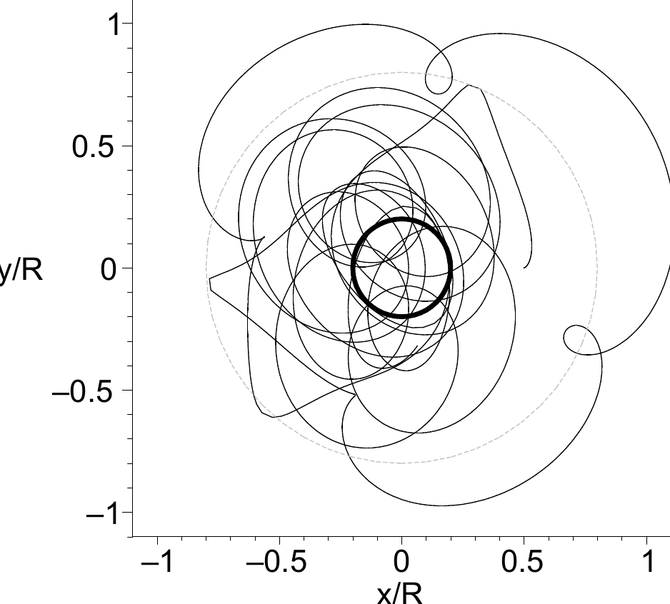
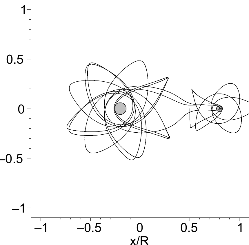
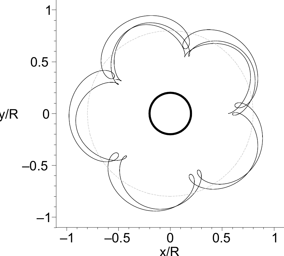
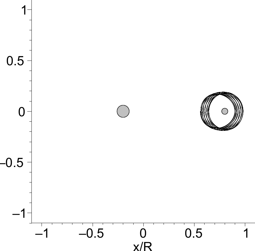
Figure 1.5 Some examples of possible trajectories in the three-body problem for different initial conditions. In all cases \(y(0) = u(0) = v(0) = 0\); \(x(0)\) is being varied. The integration time is two months. Left row: Trajectories of the earth (thick black line), moon (gray line) and satellite (thin black line), plotted in the reference frame that moves with the center of mass. Right row: Same situation as left but trajectories plotted in a reference frame that additionally co-rotates with the earth and moon. a,b] Satellite orbits around the earth. c,d] Satellite has a chaotic trajectory, orbiting both the earth and moon in a random fashion. e,f] Satellite orbits the moon. (a) \(x(0)/R = 0.3\). (b) \(x(0)/R = 0.3\). (c) \(x(0)/R = 0.5\). (d) \(x(0)/R = 0.5\). (e) \(x(0)/R = 0.56\). (f) \(x(0)/R = 0.56\).

With these substantial simplifications the order of the system has been reduced to four and does not look overly complicated, but it still cannot be analytically solved. With use of maple we can however integrate the system numerically and study the complex trajectories that occur for different initial positions and velocities of the satellite. To simplify the numerical integration a bit, we take for the mass of the moon \(m_2 = m_1/4\) instead of the real value \(m_2 = m_1/81\). Examples of trajectories for different initial conditions are given in Figure 1.5. One observes regular trajectories (orbits around the Earth or the moon) and irregular (chaotic) trajectories. Additional insight can be gained by viewing the trajectories in a reference frame that co-rotates with the circular orbit. In this view both the earth and moon have a stationary position, which simplifies the interpretation of the satellite trajectory.

A characteristic feature of chaos is the sensitive dependence on initial conditions. This feature can be nicely observed in Figure 1.6 in which two trajectories are plotted for slightly different initial conditions (relative difference 0.01%).

In the exercise you can manipulate a maple -worksheet that contains an implementation of the three-body problem (1.3). You can change the initial position and velocity of the satellite and get a feeling for the sensitivity on the initial conditions.

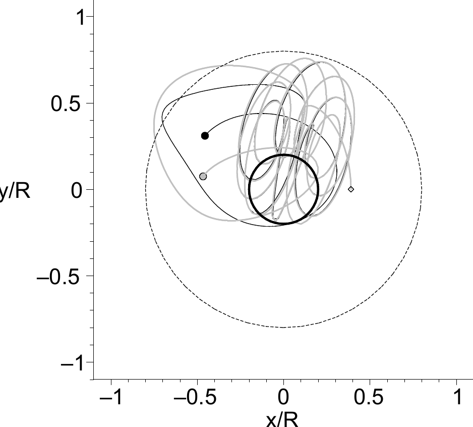
Figure 1.6 Sensitivity on initial conditions: two trajectories initiated from slightly different positions with a relative difference in \(x(0)\) of \(10^{-4}\). Integration time is two months. Diamond: initial locations. Circles: end position of satellites after two months. Top: trajectories in reference frame that moves with the center of mass. Bottom: the trajectories in the reference frame that additionally co-rotates with the earth and moon.

1.3. Exercises

1.3.1. Sensitive dependence on initital conditions in the Lorenz System

Downloads: LorenzSensitiveDependence_start.mws, LorenzSensitiveDependence.mws

Study the Lorenz system

(1.6)\[\begin{split}\begin{aligned} \dot{x} &= \sigma(y-x)\\ \dot{y} &= rx - y -xz\\ \dot{z} &= xy-bz \end{aligned}\end{split}\]

with the parameters given \(r=28,b=8/3,\sigma=10\).

Login on Blackboard/ChaoticProcesses, go to Course Documents/01 and save the file LorenzSensitiveDependence_start.mws on your computer. Start Maple Classic and load the file.

a) Execute the entire maple file once by clicking on the !!!*-button. Have a look at the time series of \(x(t)\).

b) Plot the time series of \(y(t)\) instead of \(x(t)\). (Note: you only need to slightly modify the command odeplot). Study also \(z(t)\).

c) Change the time range by modifying tstart and tend.

d) Delete the comment symbols `#‘ at the end of the file. Now you can study simultaneously the system’s behaviour for two different initial conditions. The difference between the initial values of \(x\) is \(\epsilon\). Reduce the value of \(\epsilon\) and observe the effect.

e) Reduce \(\epsilon\) until the solutions are no longer different. Increase tend to make sure. Can you understand this seemingly critical value of \(\epsilon\)?

f) Make a plot of the 3d-phase-space by plotting \([x(t),y(t),z(t)]\) instead of \([t,x(t)]\). Again you can do this with a minor change of the odeplot-command. You may want to increase numpoints as well, to get a smoother 3d-graph.

g) If everything went well you saw a so-called “strange attractor”. Why it is called strange will be dealt with later, but to see that the object is really attracting, change the initial condition \(x(0) = 2\) to \(x(0) = 100\) and look at the trajectories in phase-space. Study other initial conditions and verify that the trajectories converge upon the attractor.

1.3.2. Classification of timeseries

Downloads: ClassifyingTimeseries.mws, SomeDatasets.mws

Open the Maple file SomeDatasets.mws to view different data sets set1, set2, set3. Find out which one is a: pure random noise, b: a one dimensional mapping, c: a higher order mapping. Explain your answer.

1.3.3. Three body problem

Downloads: ThreeBody.mws, ThreeBody_start.mws, ex0036r03_fig1.pstex

Consider a satellite in space under influence of the gravitational pull of the earth and the moon.

gravitational constant	\(G\)	\(6.67 \times 10^{-11}\ Nm^2 kg^{-1}\)
distance between earth and moon	\(R\)	\(3.84 \times 10^{8}\ m\)
mass of earth	\(m_1\)	\(5.97 \times 10^{24}\ kg\)
mass of moon	\(m_2\)	\(7.36 \times 10^{22}\ kg\)

For simplicity, the orbits of earth and moon are assumed to be circular. Defining the position of the earth and moon as \(\mathbf{x}_1\) and \(\mathbf{x}_ 2\), respectively, and their mean distance as \(R\), the motion is parametrized as

\[\begin{split} \begin{gathered} \mathbf{x}_1 = -r_1 \left[ \begin{array}{c} \cos \omega t \\ \sin \omega t \end{array} \right],\ \ \mathbf{x}_2 = r_2 \left[ \begin{array}{c} \cos \omega t \\ \sin \omega t \end{array} \right], \\ r_1 = R \frac{m_2}{m_1+m_2}, \ \ \ r_2 = R \frac{m_1}{m_1+m_2}, \ \ \ \omega = 2 \sqrt{\frac{G(m_1+m_2)}{R^3} }, \end{gathered} \end{split}\]

where \(r_1\) and \(r_2\) are the radii of earth and moon, and \(\omega\) denotes the angular frequency. Using the law of gravitation \(F=G\frac{m m'}{r^2}\), the motion of the satellite is governed by

\[ \mathbf{\ddot{x}} = G m_1 \frac{\mathbf{x}_1 - \mathbf{x}} {\left|\mathbf{x}_1 - \mathbf{x}\right|^3} + G m_2 \frac{\mathbf{x}_2 - \mathbf{x}} {\left|\mathbf{x}_2 - \mathbf{x}\right|^3}. \]

Remarkably, this relatively simple system has very complex and rich behavior. The worksheet ThreeBody_start.mws contains an implementation of this system and to magnify the chaotic behavior, we have increased the mass of the moon to \(25 \%\) of the earth's mass.

a) Vary the satellite's initial position \(x_0\) in the range \([-5\cdot10^8,5\cdot10^8]\) and determine for which interval the system behaves chaotic. Study also the system in a co-rotating reference frame.

b) Check the sensitive dependence on initial conditions. Take \(x_0=2 \times 10^8\) m and set the perturbation \(\epsilon=1\) m. How many days does it take before there is a visual difference between the satellite's original and perturbed trajectory?

c) In reality the mass of the moon is a factor \(81\) lower than the earth's. If you change this, are there still chaotic trajectories? You may need to increase the initial velocity a bit.

1.3.4. Attractor reconstruction

Downloads: LorenzReconstruct.mws, LorenzReconstructStart.mws, LorenzConstruct.mws, dataset1.txt, dataset2.txt

a) Study the data set dataset1.txt, which consists of a one-dimensional time series \(xx[1]\ldots xx[N]\), “measured” with a constant sampling rate (i.e. with a constant time interval). Try to reconstruct the attractor by making a three-dimensional plot of the points \((xx[j], xx[j+\Delta j], xx[j + 2\Delta j])\), for all possible \(j\). The maple command spacecurve may be useful in this respect. See also the file LorenzReconstructStart.mws. Change \(\Delta j\) to get the best result.

b) Do the same for dataset2.txt, which has some additional noise superimposed.