2. The physics behind the Lorenz equations

The Lorenz equations studied in 6 were simply stated there as a celebrated example of a chaotic flow. The purpose of this appendix is to show where they come from: far from being an abstract construction, they are a drastically truncated model of thermal convection. Following the derivation also gives a physical meaning to the three variables \(x\), \(y\), \(z\) and to the parameters \(\sigma\), \(r\) and \(b\).

The Hungarian mathematician George Polya (1887–1985) once said: “If you can't solve a problem, then there is an easier problem you can solve: find it.” In this spirit, Ed Lorenz initiated the revolution of chaos theory with his seminal paper titled “Deterministic Nonperiodic Flow” [Lorenz, 1963]. Lorenz was interested in the predictability of weather forecasting. Instead of attempting to solve the immensely complex system of three-dimensional partial differential equations governing the atmosphere, he stripped away all detail until he was left with only three ordinary differential equations, which now carry his name.

2.1. Rayleigh–Bénard convection

The model Lorenz considered was a layer of air confined between two flat plates, heated from below and cooled from above. This flow is known as Rayleigh–B'{enard convection}. It may seem a far stretch from weather prediction, but it shares some essential features. The heating from below resembles the heating of the earth's surface by solar radiation during the day. As hot air is lighter than cold air, it rises due to its buoyancy, forming thermals – pockets of rising hot air – that birds and glider pilots gratefully use to stay airborne for extended periods. In the atmosphere, thermals transport not only heat but also water vapour to the free troposphere, making them of primary importance to the hydrological cycle and thus to weather prediction. Rayleigh–Bénard convection has these thermals too (Figure 2.25): if there is a predictability problem in this simplified system, one can be certain that it will also be present in the far more complex atmosphere.

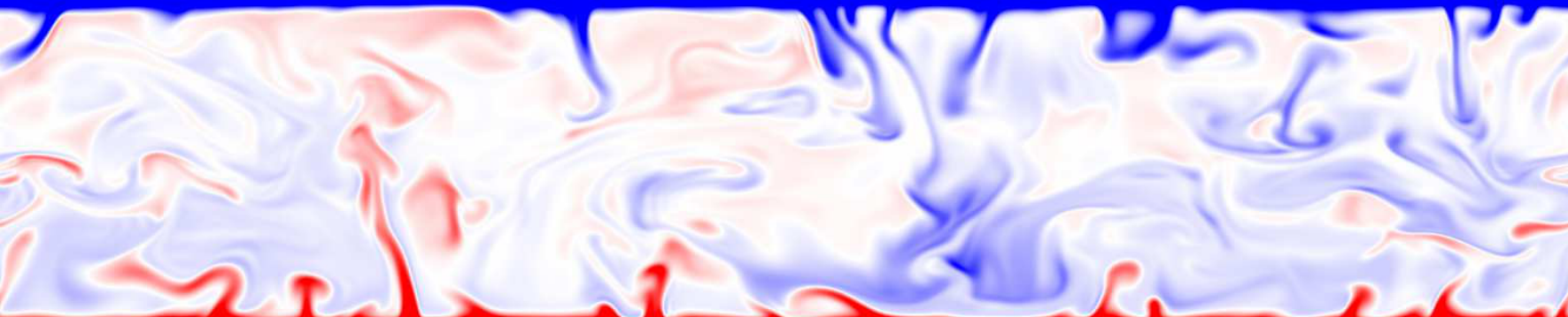
Figure 2.25 A snapshot of the temperature field of Rayleigh–Bénard convection obtained by direct numerical simulation, in which the turbulence is resolved down to the smallest scales.

Rayleigh–Bénard convection

Under the Boussinesq approximation, the velocity field \(\mathbf{u}\), pressure \(p\) and temperature deviation \(\Theta\) of the convecting layer obey conservation of mass, momentum and energy,

\[\begin{split} \begin{gathered} \nabla \cdot \mathbf{u} = 0, \\ \frac{\partial \mathbf{u}}{\partial t} + \mathbf{u} \cdot \nabla \mathbf{u} + \frac{1}{\rho} \nabla p - \nu \nabla^2 \mathbf{u} = \beta \mathbf{g}\, \Theta, \\ \frac{\partial \Theta}{\partial t} + \mathbf{u} \cdot \nabla \Theta - \kappa \nabla^2 \Theta = 0, \end{gathered} \end{split}\]

where \(\rho\) is the density, \(\nu\) the kinematic viscosity, \(\kappa\) the thermal diffusivity, \(\beta\) the thermal expansion coefficient and \(\mathbf{g}\) gravity. Resolving these equations down to the smallest scales – a direct numerical simulation (Figure 2.25) – is enormously demanding [Hanjalić, 2005, Heslot et al., 1987, van Reeuwijk et al., 2006]; the Lorenz equations arise from the opposite extreme, retaining only the very largest scales of motion.

2.2. From convection to three equations

Starting from the convection equations above, Lorenz considered the two-dimensional instability and expressed the fields with a Galerkin method [Holmes et al., 1996, Saltzman, 1962] as an infinite sum of Fourier modes. Retaining only the lowest-order modes leaves three time-dependent amplitudes \(x(t)\), \(y(t)\) and \(z(t)\) that nonetheless characterise an entire velocity and temperature field,

(2.50)\[\begin{split}\begin{gathered} u(x, z, t) = -x(t)\, \frac{(1+a^2)\pi}{a}\, \sin(\pi a x)\cos(\pi z), \\ w(x, z, t) = x(t)\, \pi (1+a^2)\, \cos(\pi a x)\sin(\pi z), \\ \Theta(x, z, t) = \frac{1}{r\pi}\Bigl( y(t)\cos(\pi a x)\sin(\pi z) - \tfrac{1}{2} z(t)\sin(2\pi z)\Bigr) - \bigl(z - \tfrac{1}{2}\bigr). \end{gathered}\end{split}\]

The key point is that these expressions are factorised: all time dependence resides in \(x\), \(y\) and \(z\), while the spatial dependence is carried entirely by the trigonometric terms. Physically, \(x(t)\) controls the strength of the convective velocity field; \(y(t)\) represents the temperature difference between ascending and descending air; and \(z(t)\) measures the deviation of the temperature profile from the linear conduction profile \(\Theta(z) = -(z - \tfrac{1}{2})\). A representative flow field described by ((2.50)–(2.50)) is shown in Figure 2.26.

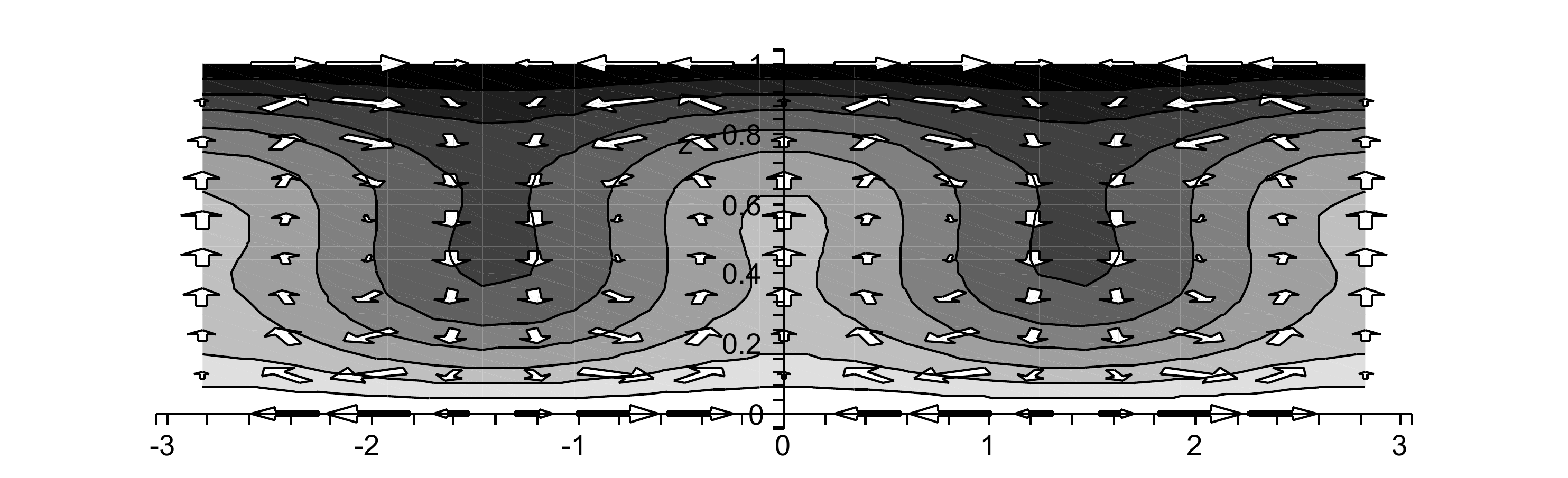
Figure 2.26 The velocity and temperature field that the variables \(x\), \(y\) and \(z\) describe.

Substituting ((2.50)–(2.50)) into the momentum and temperature equations and neglecting the interactions with the higher-order modes that were dropped, these three amplitudes are found to obey the closed system

\[\begin{split} \begin{aligned} \dot{x} &= \sigma (y - x), \\ \dot{y} &= r x - y - x z, \\ \dot{z} &= x y - b z. \end{aligned} \end{split}\]

The parameter \(r\) is a non-dimensional temperature difference which drives the flow; the Prandtl number \(\sigma\) is the ratio of kinematic viscosity to thermal diffusivity; and \(b\) is a measure of the aspect ratio of the convection rolls, a large value corresponding to a low aspect ratio and vice versa. It should be stressed that this truncation describes only the onset of instability in Rayleigh–Bénard convection, and is quantitatively faithful only near the convective threshold. Remarkably, however, the very same equations describe other physical systems exactly, among them a mechanical waterwheel [Strogatz, 1994] as well as certain lasers and dynamos.

It was in this system that Lorenz encountered what seemed, in the early sixties, a genuine paradox. The term deterministic was then associated with systems whose long-term fate was to settle onto a fixed point or a limit cycle, whereas nonperiodic behaviour was associated with random forcing. Yet here the trajectories remained confined to a bounded region of phase space while every small volume of initial conditions was flattened towards zero volume, and Lorenz could show that the system possessed neither a stable fixed point nor a stable limit cycle. He was forced to conclude that the flow was at once deterministic and nonperiodic – he had stumbled upon a strange attractor.