4. Continuous Systems#
4.1. Fixed points and stability#
A first-order continuous autonomous system is given by
where \(\dot{x} = \mathrm{d} x/\mathrm{d} t\). An example is
The word autonomous means that the right-hand of (4.1) has no explicit time dependence; the dependence on time is implicit through the variable \(x\), i.e. \(f(x(t))\). For non-autonomous systems the explicit time-dependence is indicated separately
An example of a non-autonomous system is
Below we will deal with autonomous systems only.
An analytical solution to (4.1) may be sought by the following approach
where \(c\) is an integration constant which will be determined by the initial condition \(x(0)\). The success of the method depends on whether one can find an analytical solution to the integral over \(x\). As an example, consider
Following (4.5) we are to solve
One can rewrite the fraction in three separate terms
where the constants \(A,B,C\) can be found by elaborating the expression at the right-hand side
Working out the numerator and collecting terms with \(x,x^2\) and no \(x\) separately, one obtains three equations from which \(A,B,C\) can be determined
hence \(A = 1, B = 1/2, C = -1/2\) and one can proceed to integrate (4.7):
Inverting the last terms and using the initial condition \(x(0)=x_0\), one gets an expression for \(x\) directly in terms of \(t\) and \(x_0\)
The following commands make use of maple's ability to find analytical solutions:
Maple
restart: with(plots):
f := x->x-x^3;                   # define f(x)
eq:=diff(x(t),t)=f(x(t));        # define differential eq
sol:=dsolve({eq,x(0)=x0},x(t));  # solve it analytically
x0 := 0.1;                       # set initial condition
plot(rhs(sol),t=0..6);           # plot the solution
Yet in many cases you (or maple) will not be so fortunate to find an analytical solution for \(x(t)\). This is either because one cannot evaluate the integral \(\int [f(x)]^{-1} \mathrm{d} x\), or because one cannot invert the result which is required to get \(x\) expressed as a function of \(t\).
An example, relevant to physics, is
where \(T\) is a parameter. This equation describes the evolution of the magnetization of a ferromagnetic system at temperature \(T\). The problem here is that one cannot find an expression for the integral \(\int [-x+\tanh(x/T)]^{-1} \mathrm{d} x\). We will deal with this system later in more detail.
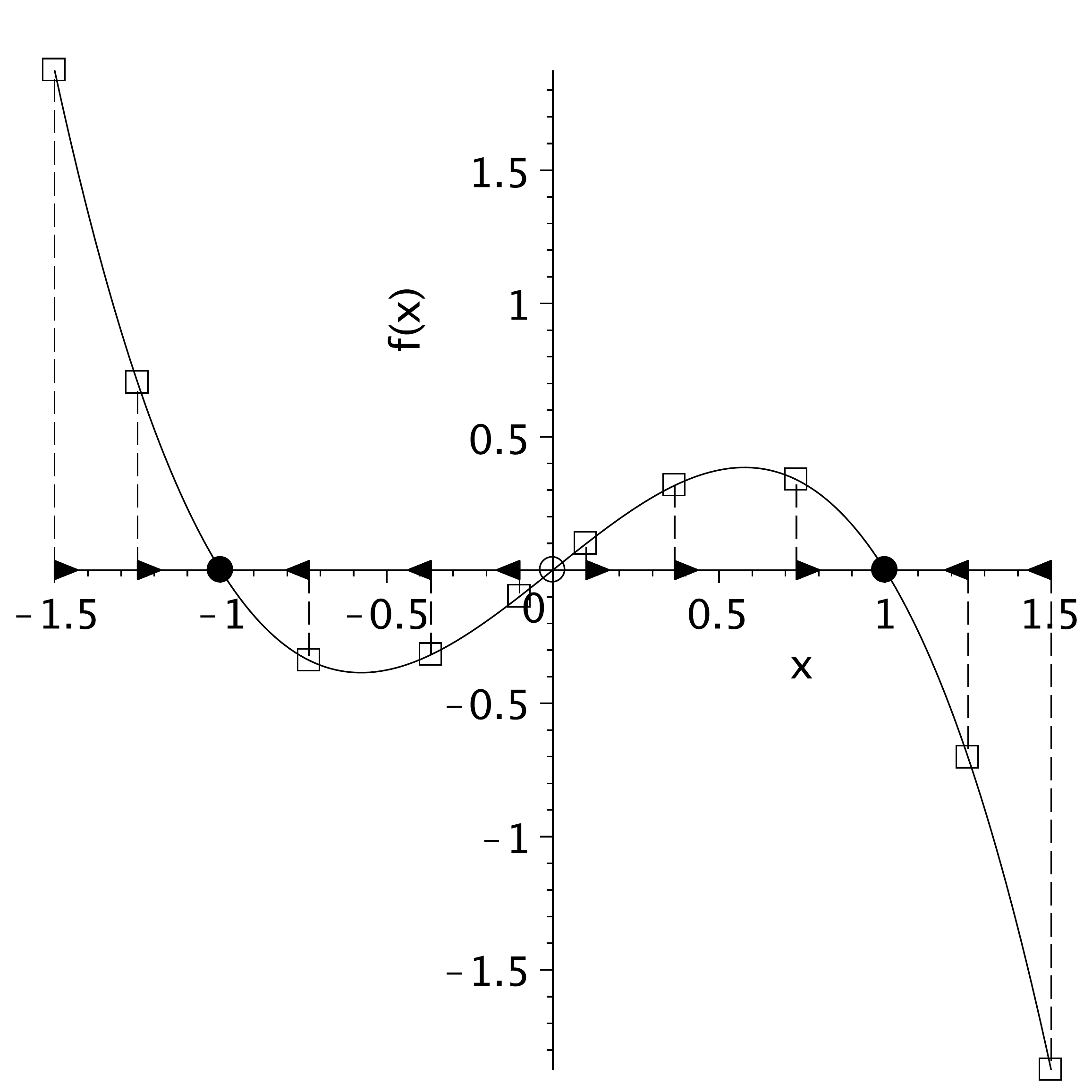
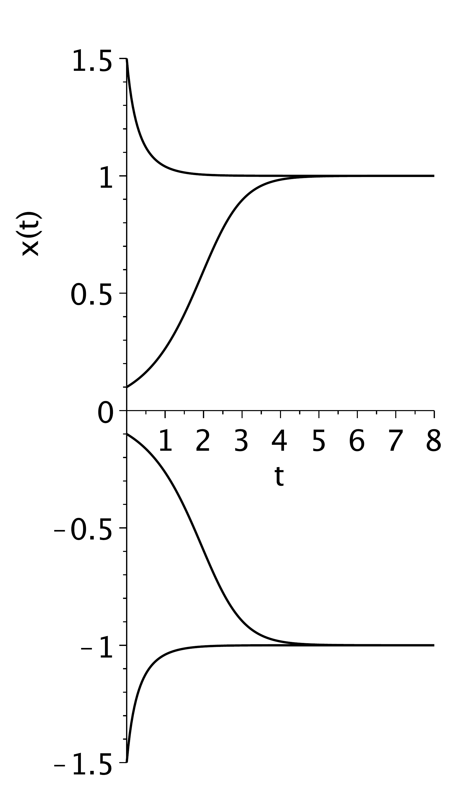
Figure 4.1 Graphs for the system \(\dot{x}=f(x)=x-x^3\). (a) Graph of \(f(x)=x-x^3\). (b) Evolution of \(x\) from four initial conditions.#
Fortunately it is still possible to get a good understanding of the behaviour of the system even in absence of closed form analytical solutions. Let us revisit example (4.6). A plot of \(f(x) = x-x^3\) is shown in Figure 4.1. What happens with the evolution of \(x(t)\) when you start at \(x(0) = 1.5\)? The rate of change, \(\dot{x}\), at this point is given by \(f(1.5)\). Looking at the graph in Figure 4.1 one sees that \(f(1.5) < 0\), hence the rate of change is negative, which means that \(x\) will decrease (as indicated by the arrow on the \(x\)-axis). While \(x\) decreases, the rate of change \(\dot{x}=f(x)\) still remains negative, so \(x(t)\) continues to decrease until \(x=1\) has been reached. At this point the rate of change has become zero, \(\dot{x}= f(1) = 0\), so \(x\) will no longer change. If on the other hand one starts at, say, \(x_0=0.1\), one finds \(f(0.1)>0\) implying that \(x\) will increase (indicated by the arrow pointing to the right). Since \(f(x)\) remains positive, \(x\) increases until it again arrives at \(x=1\) where the rate of change is zero. Such points where \(\dot{x} = 0\) are called fixed points.
Fixed points can be readily located by detecting where the graph of \(f(x)\) crosses the \(x\)-axis. Looking at Figure 4.1 one notices three fixed points \(x_* = -1,\,x_* =0\) and \(x_* =1\), respectively. The fixed point \(x_* = 0\) differs from the other two because it is unstable. If one starts exactely at \(x(0) = x_* = 0\) then also \(x(t) = 0\) for all \(t>0\). But a slight perturbation will cause \(x\) to evolve towards one of the stable fixed points \(x_* = \pm 1\).
The set of initial conditions that lead to a certain fixed point is called the domain of attraction of that fixed point. In the example the attraction domain of \(x_*=1\) is \(\langle 0,\infty\rangle\), and that of \(x_*=-1\) is \(\langle -\infty,0\rangle\). The unstable fixed point \(x_*=0\) has no attraction domain by definition.
The graphs in Figure 4.1, which represent the numerical solution to (4.6) for different initial conditions, were made using the following maple commands
Maple
restart: with(plots):
f := x->x-x^3;                                # define f(x)
eq:=diff(x(t),t)=f(x(t));                     # define differential eq
sol:=dsolve({eq,x(0)=0.1},x(t),type=numeric); # solve it numerically
odeplot(sol,[t,x(t)],0..6);                   # plot the solution
There was of course no need to employ a numerical procedure since we already had derived the analytical solution (4.8) (which yield the same graphs), but, as mentioned above, having an analytical solution at ones disposal does not happen often, which is why the numerical version is probably more useful in general.
Apart from the numerical/analytical solution, one could have made a sketch of the evolution onseself based solely on the graph of \(f(x)\) in Figure 4.1: take for instance the evolution starting at \(x_0=0.1\). Initially the rate of change is only moderately positive, but as \(x(t)\) slowly increases to larger values also \(f(x)\) becomes larger, thus speeding up the increase. As \(x\) gets closer to \(x_* = 1\), the rate of change decreases and the convergence to 1 slows down and ultimately comes to a halt at \(x=1\). In this way one can qualitatively well understand the evolution trajectories of Figure 4.1.
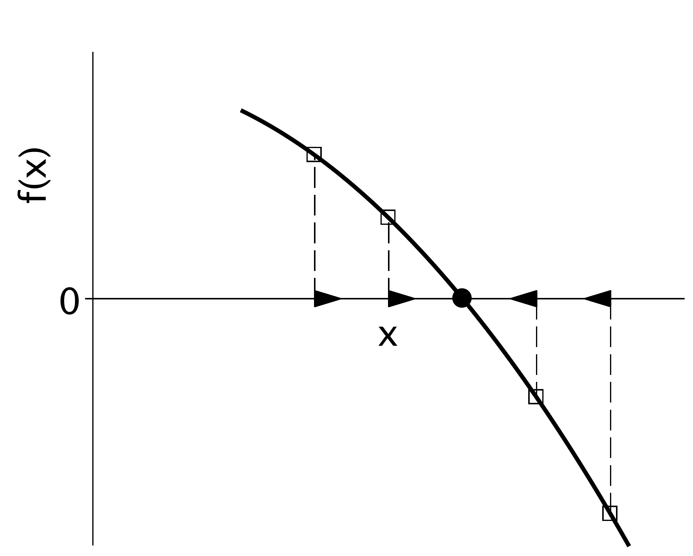
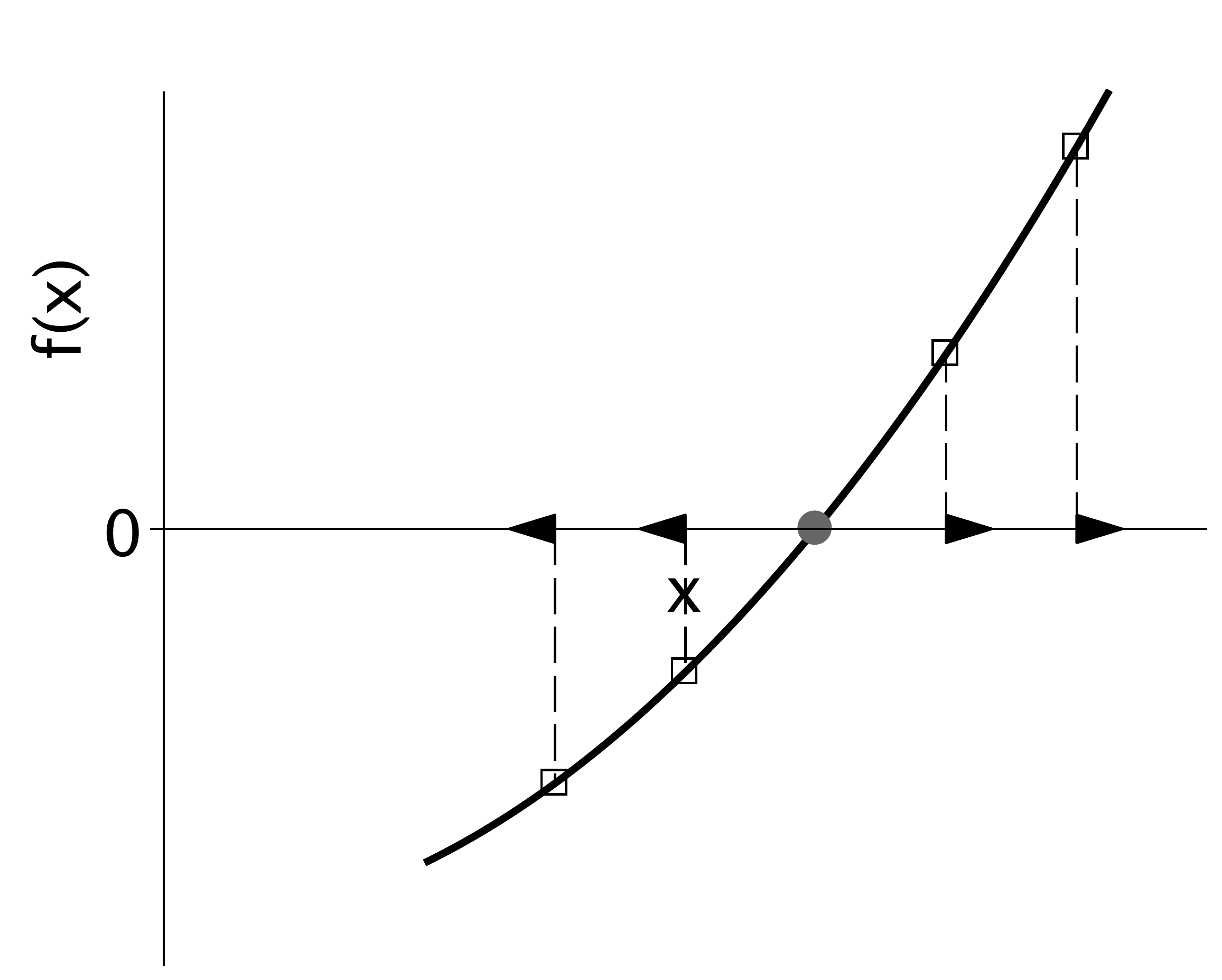
Figure 4.2 Stable and unstable fixed points. (a) Stable fixed point: \(f'(x_*)<0\). (b) Unstable fixed point: \(f'(x_*)>0\).#
The graphical method outlined above works well for arbitrary systems \(\dot{x} = f(x)\). First one makes a graph of \(f(x)\) and locates the zero crossings to find the fixed points. If a zero-crossing looks similar to Figure 4.2, in the sense that if the derivative of \(f\) with respect to \(x\) evaluated in the fixed point is negative, one deals with a stable fixed point. If the derivative is positive \(f'(x_*)\), such as depicted in Figure 4.2, the fixed point is unstable. Below we will put this issue on a firmer footing.
4.1.1. Local stability analysis of fixed points#
Here we pursue a more mathematically oriented approach to determine the stability of fixed points to \(\dot{x}=f(x)\). As said, a fixed point \(x_*\) satisfies
To investigate the stability of a fixed point, put the system in the fixed point and apply a perturbation \(x(0) = x_* + \epsilon(0)\), where \(\epsilon(0)\ll 1\). To see whether the system will return to the fixed-point, or whether it will diverge even further from it, one is interested in the evolution of the deviations from the fixed point: \(\epsilon(t) = x(t) - x_*\). Differentiation with respect to \(t\) followed by a Taylor expansion gives
with \(f' = \mathrm{d} f/\mathrm{d} x\). The first term at the right is zero because of (4.9). Neglecting the higher-order terms in \(\epsilon\), one is left with \(\dot{\epsilon} = \epsilon f'(x_*)\). Since \(\sigma = f'(x_*)\) is constant, the solution for \(\epsilon(t)\) is given by
Requiring \(\epsilon(t) \rightarrow 0\) yields the condition \(\sigma < 0\). Hence we conclude
which is consistent with Figure 4.2.
Let us apply this to example (4.6). The derivative is \(f'(x) = 1 - 2x^2\), so for \(x_* = \pm 1\) one has \(\sigma = -1\), demonstrating that both fixed points are stable. For \(x_* = 0\), one gets \(\sigma = 1\) hence it is unstable.
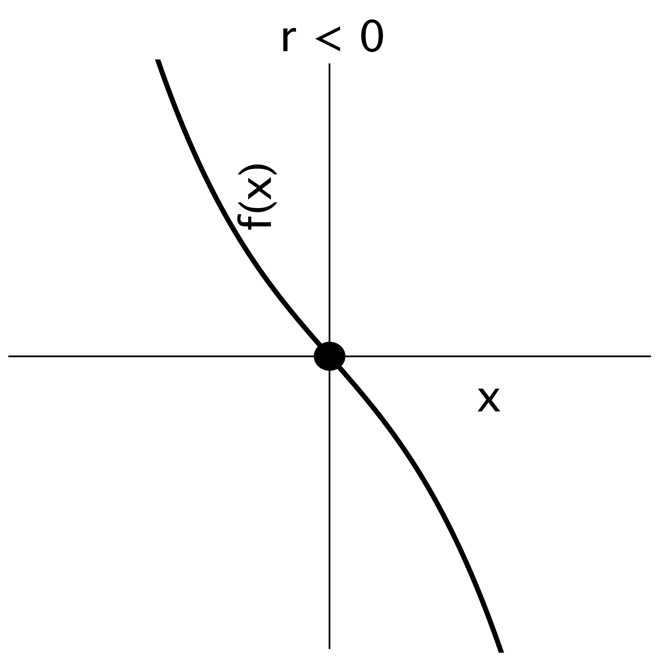
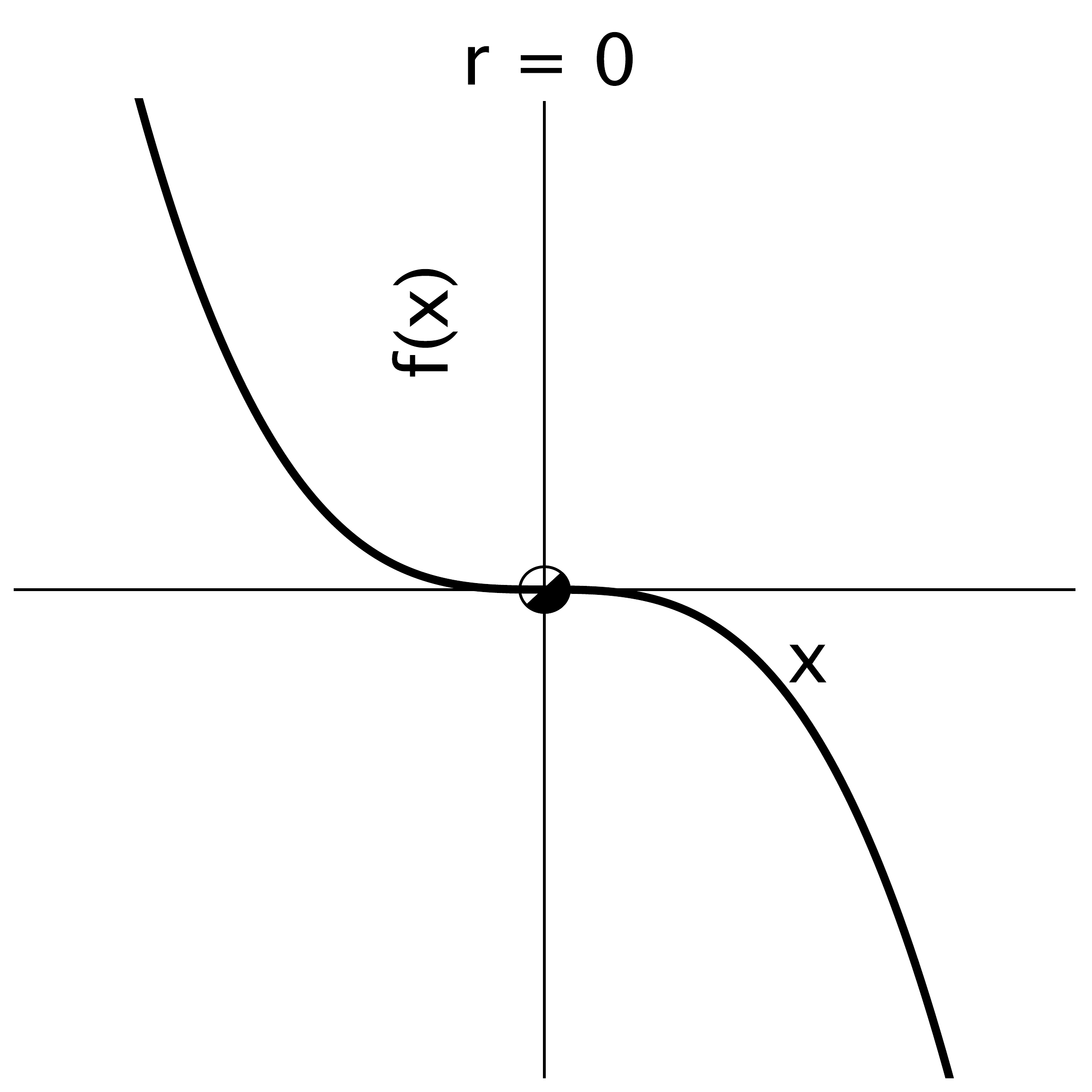
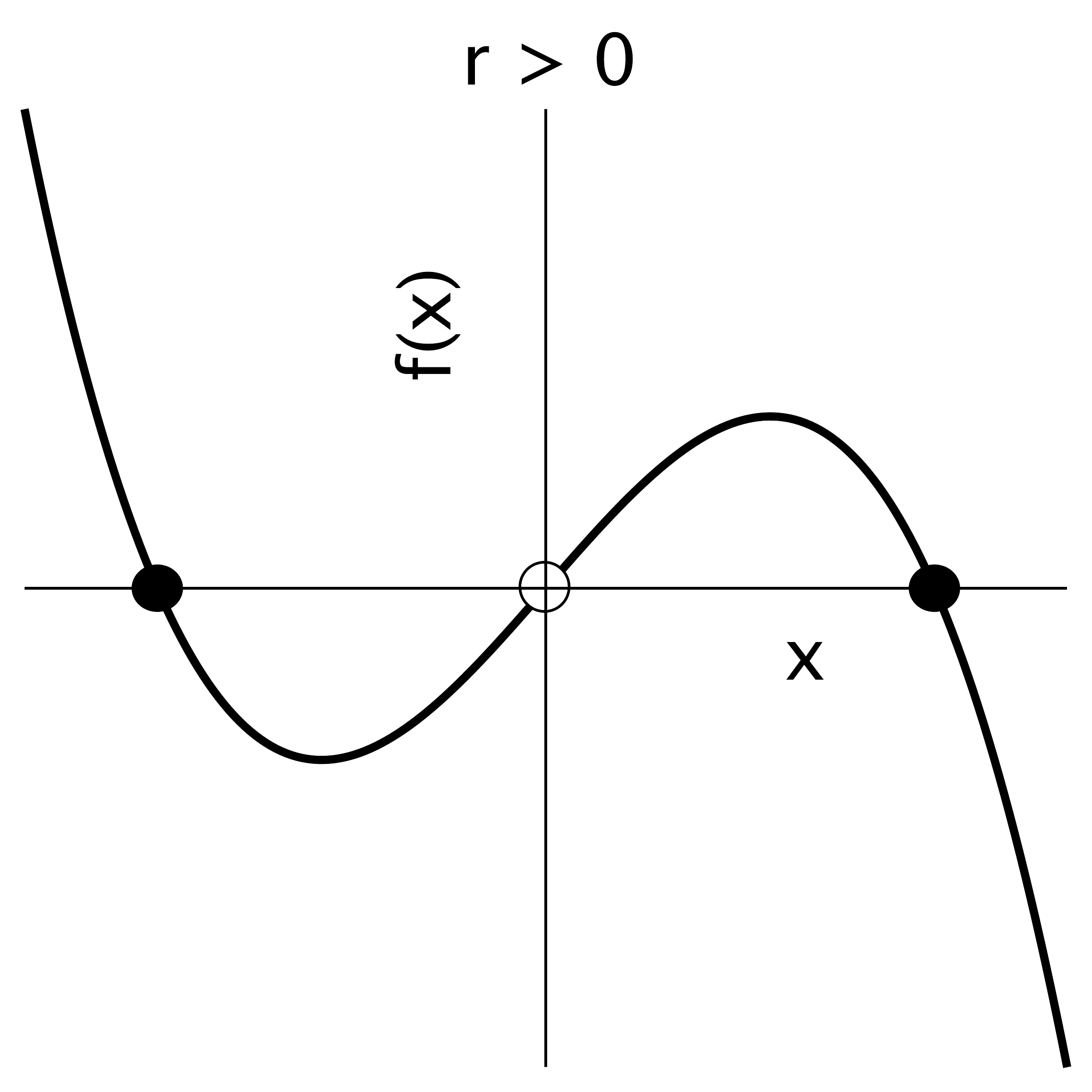
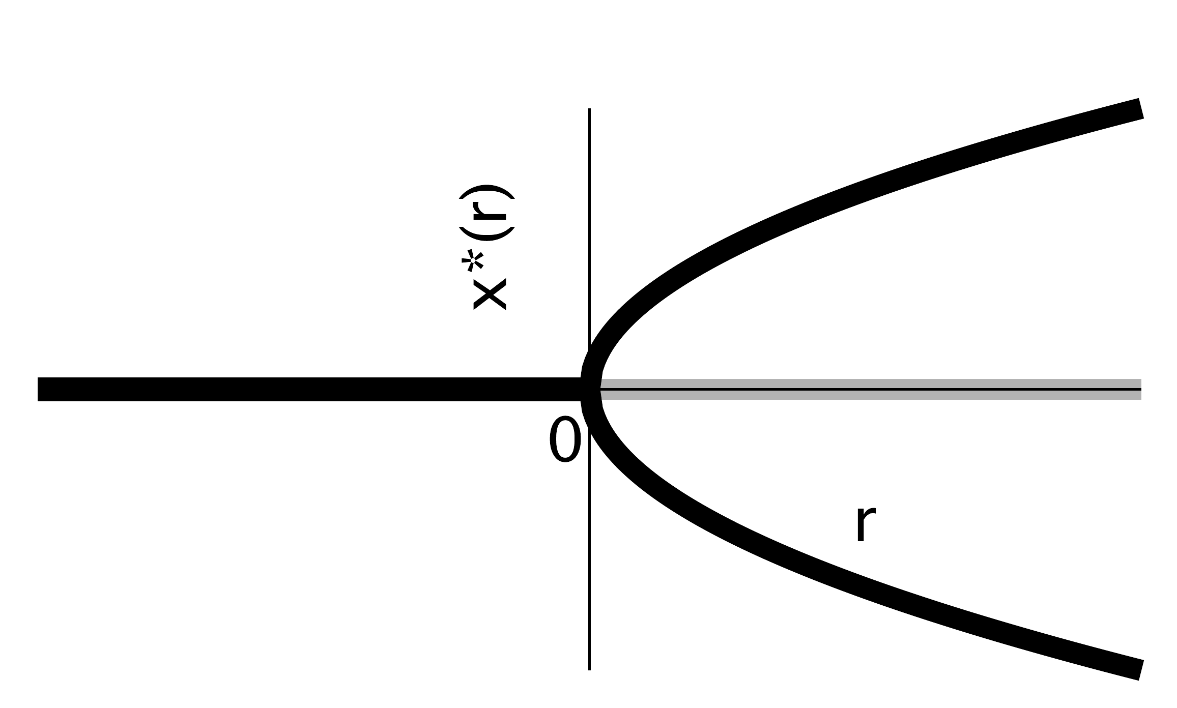
Figure 4.3 Pitchfork bifurcation in \(\dot{x} = rx- x^3\). The bifurcation diagram in (d) corresponds to graphs (a)-(c). A black color means that the fixed point branch \(x_*(r)\) is stable, whereas gray means unstable. (d) Bifurcation diagram.#
4.2. Pitchfork bifurcation#
A bifurcation is the process where one or more fixed points are created or annihilated due to changes in an external parameter of the system. It turns out that the number of commonly occuring bifurcation types is limited. Apparently there is only a limited number of possibilities to create or destroy fixed-points. We treat the three most common ones below.
As an example, let us add a parameter \(r\) to the system (4.6):
where \(r\) can be positive or negative (or zero). Sketches of \(f_r(x)\) for various \(r\) are given in Figure 4.3. One observes that for \(r<0\) there is a single fixed point \(x_* = 0\) which is stable. At \(r=0\) the stability of this fixed point changes and becomes unstable for \(r>0\). However, also two new (stable) fixed points have been created. Solving for \(f(x_*)=0\) gives an expression for the fixed points as a function of \(r\); the stability is then given by \(\sigma = f_r'(x_*) = r - 3x_{*}^{2}\):
These three branches have been plotted in Figure 4.3. The \(x_*(r) = 0\) branch changes stability around \(r=0\) (indicated by the color change from black to gray). This type of bifurcation is called a pitchfork bifurcation – 'bifurc' is the Latin word for fork.
4.3. Saddle-node bifurcation#
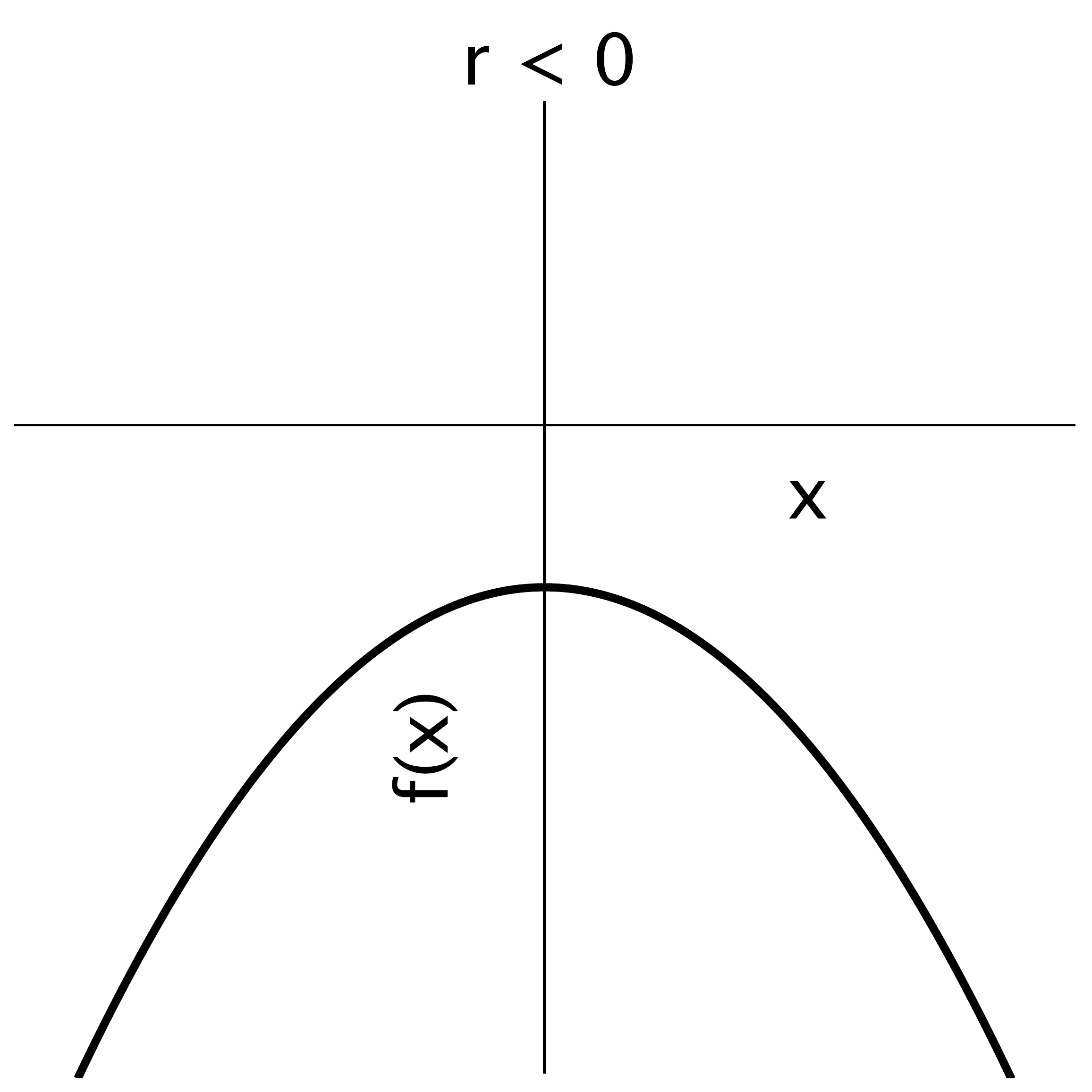
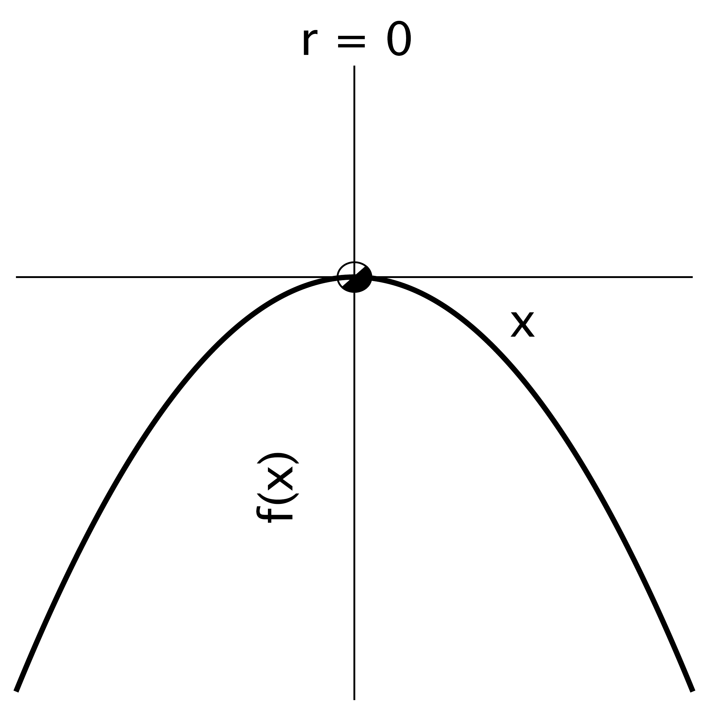
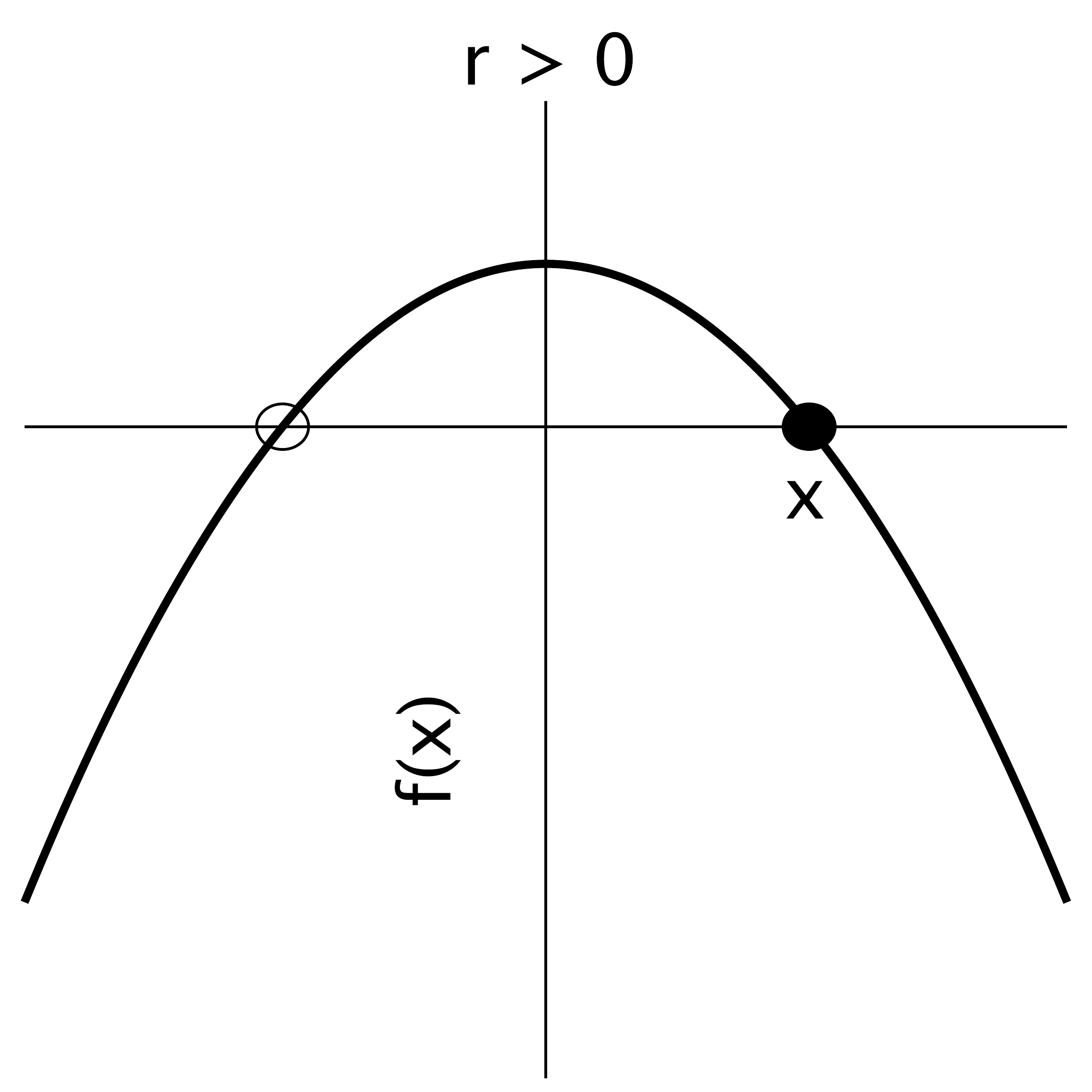
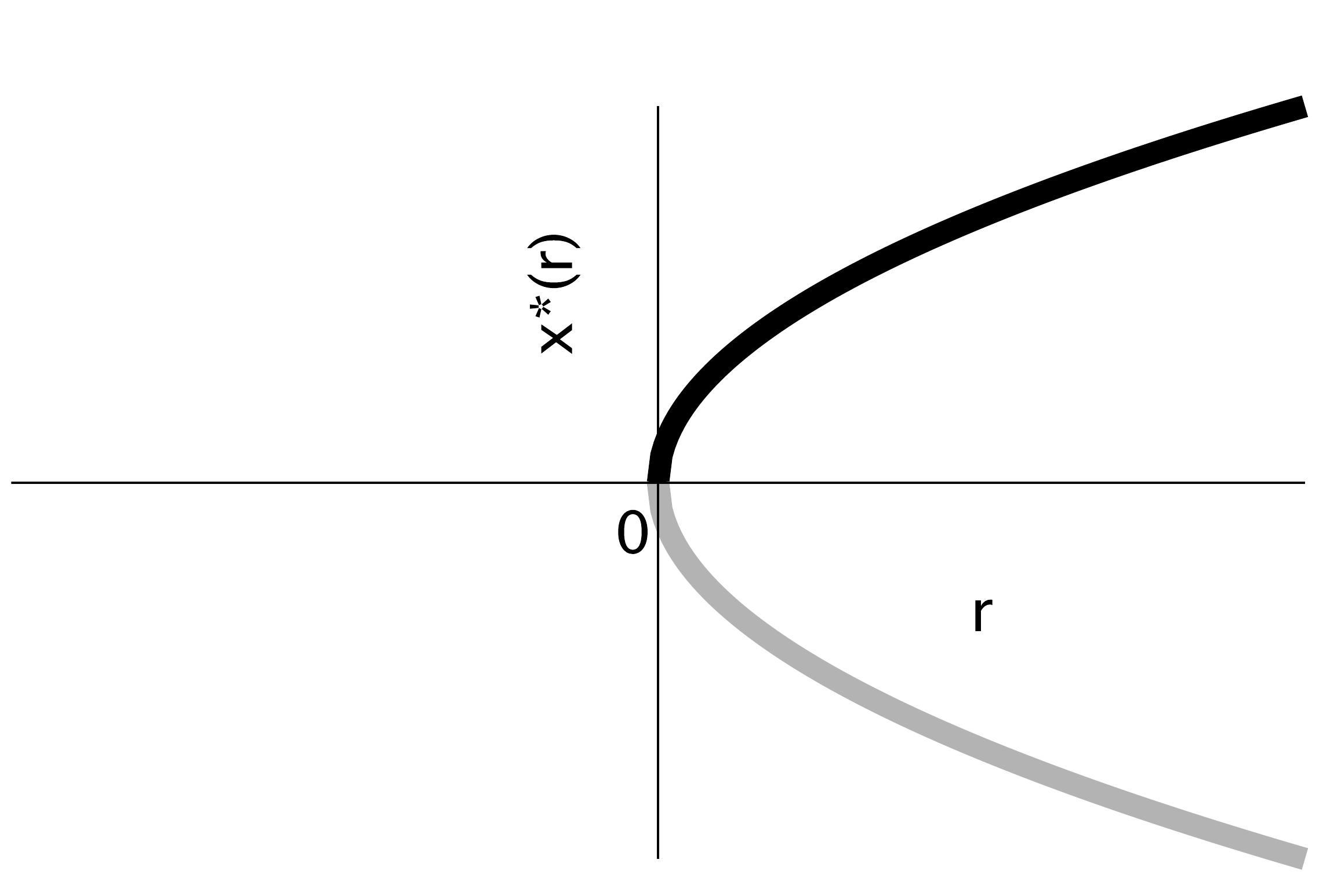
Figure 4.4 Saddle node bifurcation in \(\dot{x} = r - x^2\). The bifurcation diagram in (d) corresponds to graphs (a)-(c). A black color means that the fixed point branch \(x_*(r)\) is stable, whereas gray means unstable. (d) Bifurcation diagram.#
A so-called saddle-node bifurcation is associated with
The corresponding plots for various \(r\) are displayed in Figure 4.4. For \(r<0\) there is no fixed point, but the situation changes at \(r=0\), as for \(r>0\) two fixed points have been created simultaneously, one stable and one unstable. The fixed points are \(x_*(r) = \pm \sqrt{r}\). The stability follows from \(\sigma = f_r'(x_*) = -2x_*\):
The branches have been plotted in Figure 4.4. Note the essential differences with the pitchfork bifurcation displayed in Figure 4.3: there are no fixed points for \(r<0\), but when \(r\) changes sign two fixed points are created 'out of the blue', a stable and an unstable one.
4.4. Transcritical bifurcation#
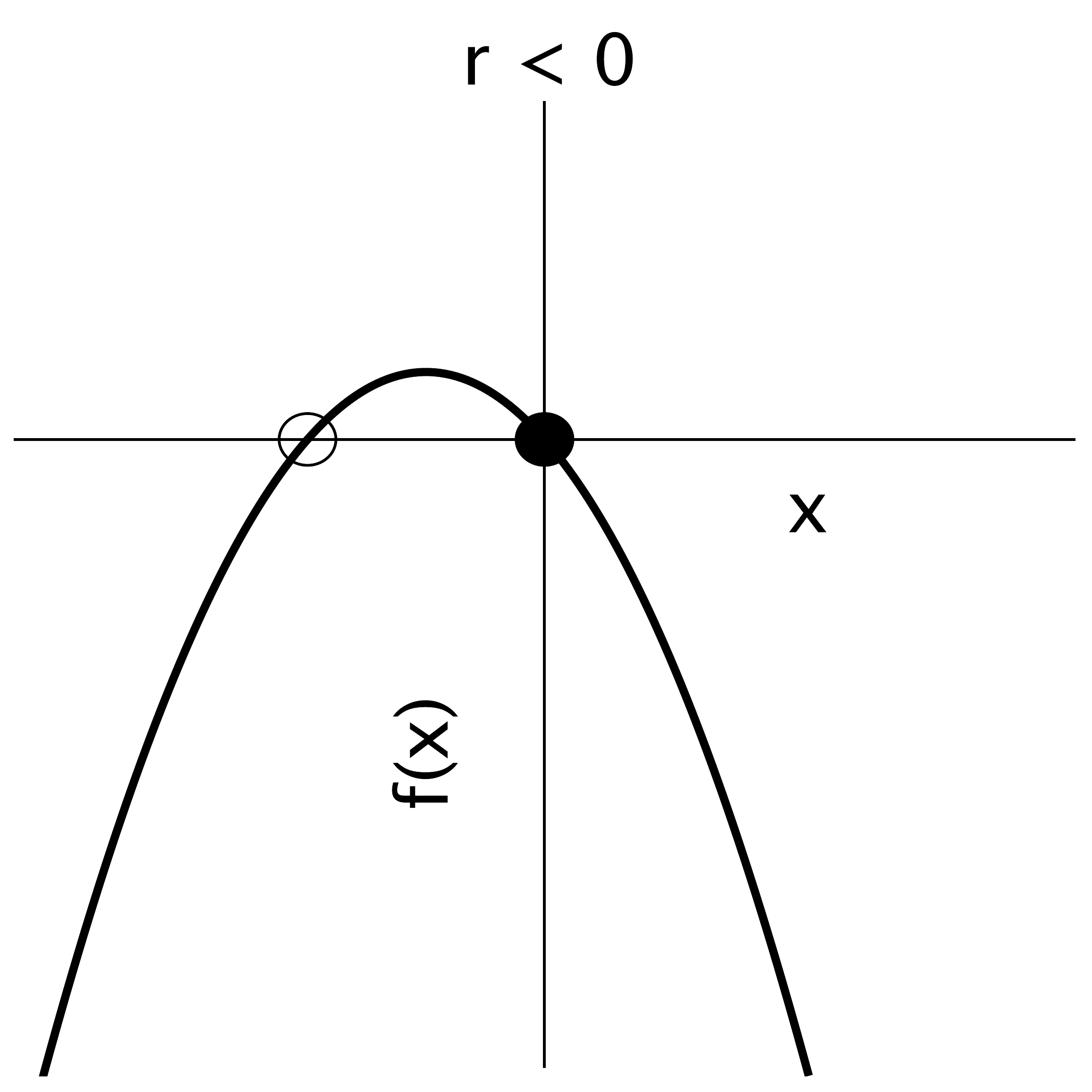
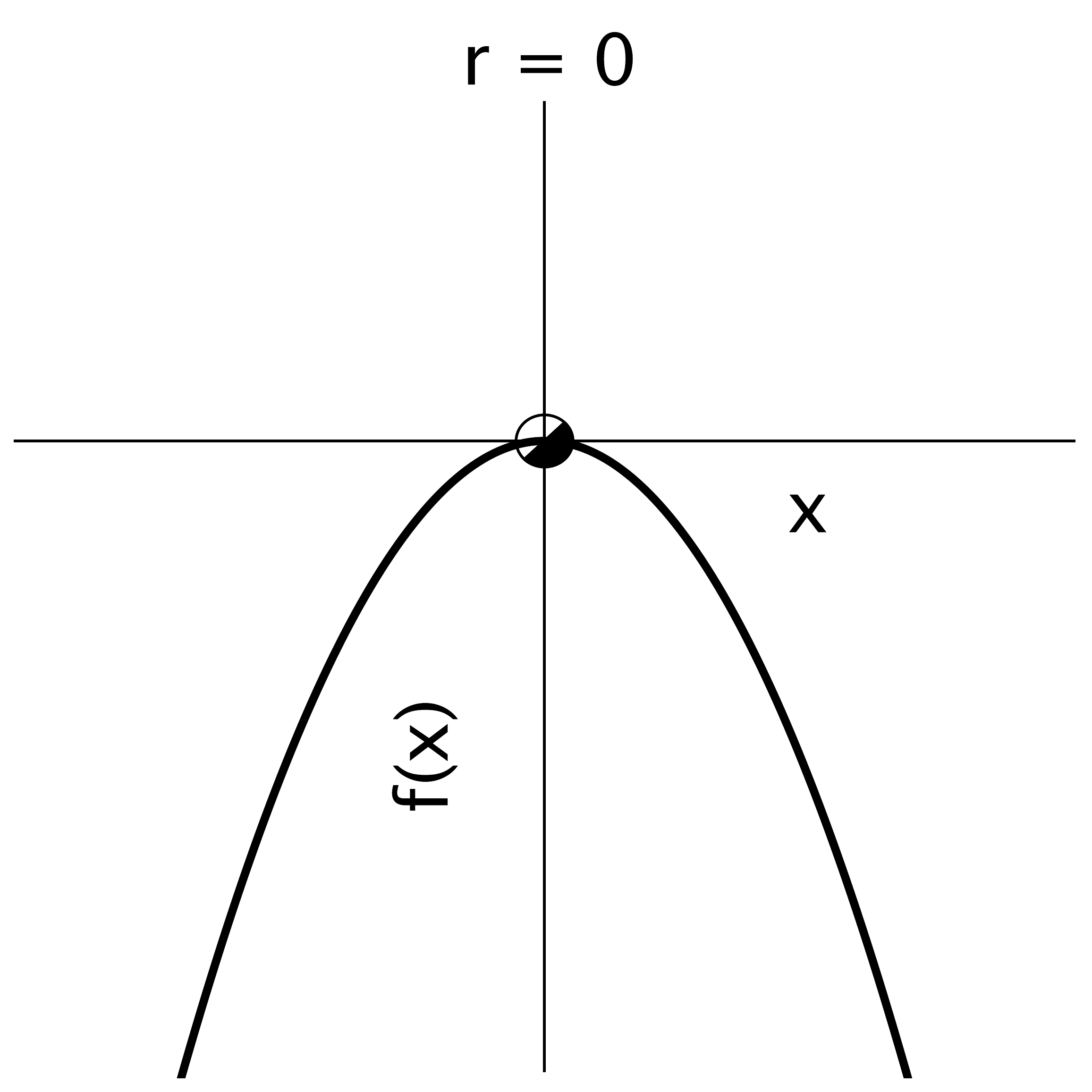
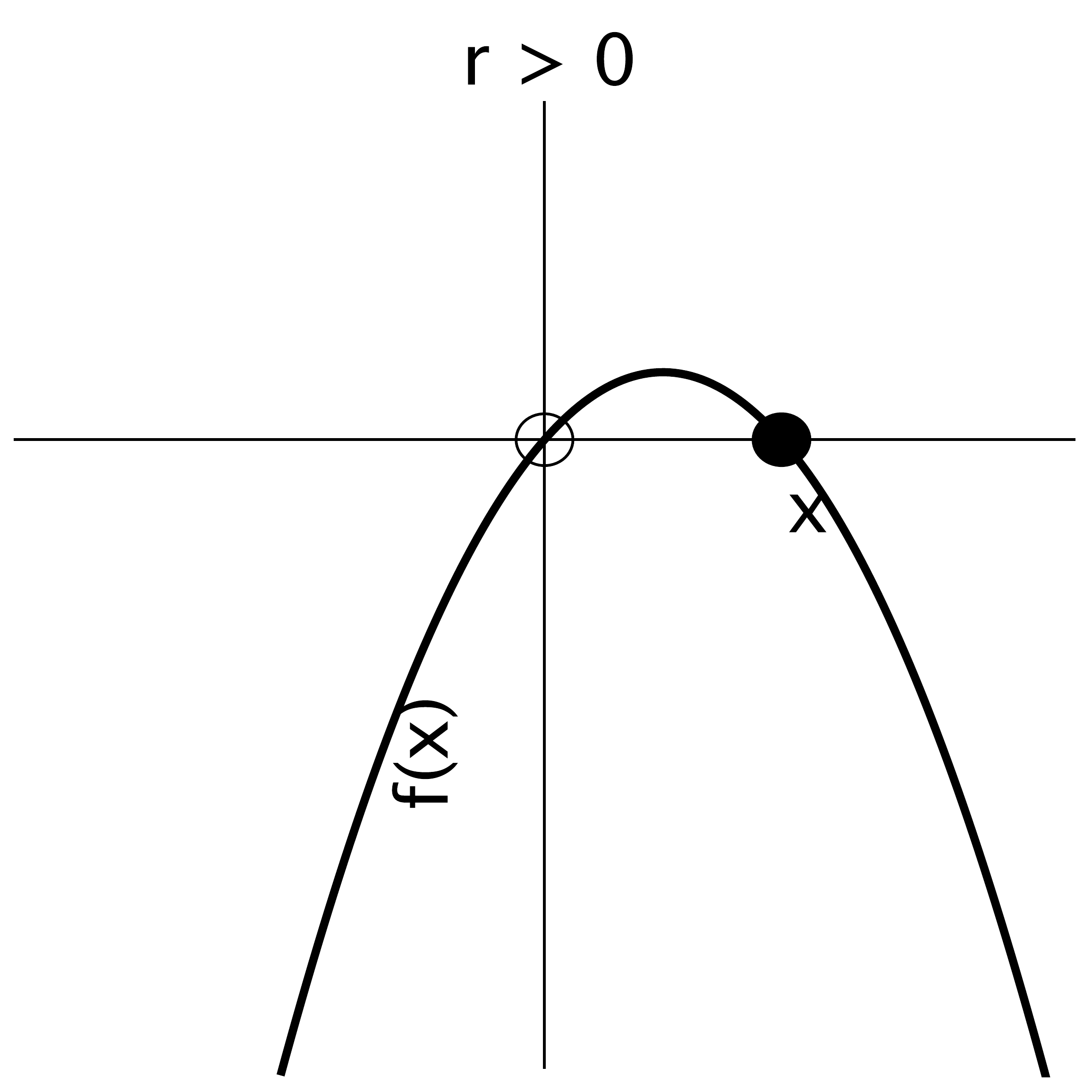
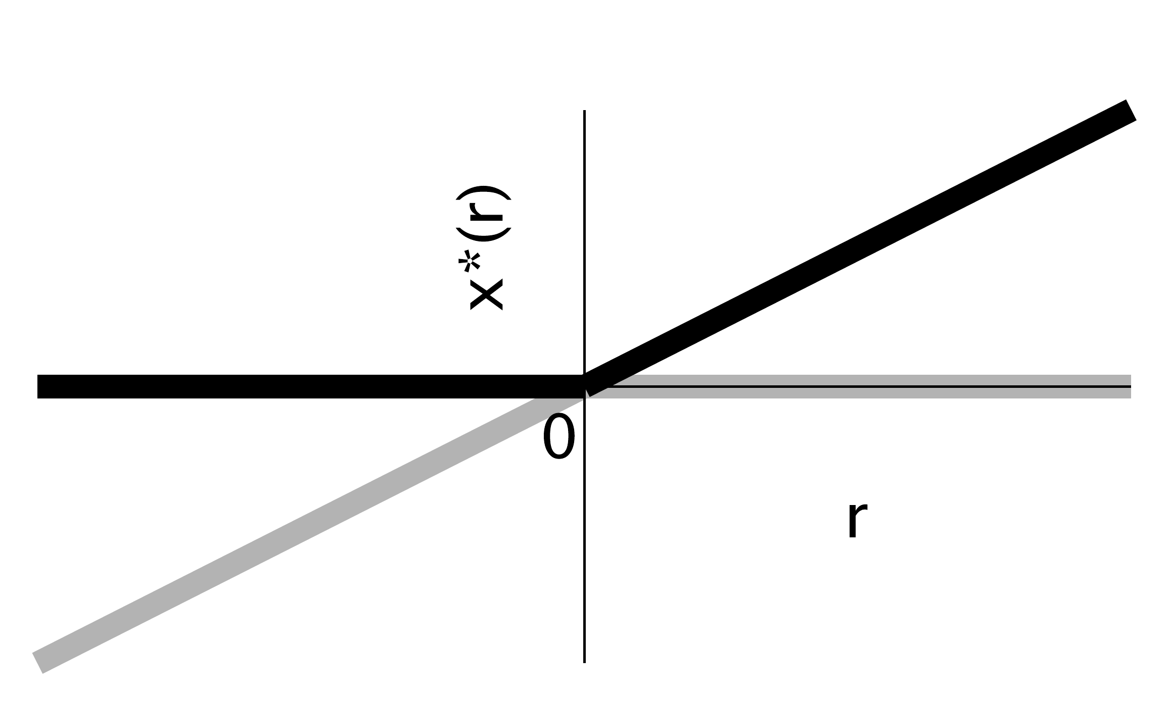
Figure 4.5 Transcritical bifurcation in \(\dot{x} = rx - x^2\). The bifurcation diagram in (d) corresponds to graphs (a)-(c). A black color means that the fixed point \(x_*(r)\) is stable, whereas gray means unstable. (d) Bifurcation diagram.#
The third type is called transcritical bifurcation, associated with a system of the form
The fixed points follow from \(f_r(x_*)=0\), and the stability from \(\sigma = f_r'(x_*) = r-2x_*\)
The corresponding plots are given in Figure 4.5: one observes that the branches exchange their stability around \(r=0\). This 'exchange of stability' characterizes a transcritical bifurcation.
4.5. Universality of bifurcations: normal forms#
Although the number of one-dimensional non-linear autonomous systems is infinite, the idea is that commonly only a limited number of bifurcation types occur. The underlying reason is that close to the bifurcation point, the system can be well approximated by the first terms of a Taylor series, of which only a few forms are most likely to occur. Consider the generic autonomous system \(\dot{x} = f(x,\mu)\) which undergoes a bifurcation at \(\mu=\mu_c\). The fixed point(s) around bifurcation \(x_*(\mu)\) satisfy \(f(x_*,\mu)=0\). The stability is \(\sigma = f'(x_*(\mu),\mu)\). Let \(x_c = x_*(\mu_c)\). Precisely at the bifurcation \(\sigma = f'(x_c,\mu_c)=0\). Expanding \(f(x,\mu)\) via a Taylor series in \(x\) and \(\mu\) around \((x_c,\mu_c)\)
The first two terms are zero. Defining \(y=x-x_c\) and \(\nu = \mu-\mu_c\) gives
where \(a= \frac{\partial f}{\partial \mu}(x_c,\mu_c)\), \(b=\frac{\partial^2 f}{\partial x \partial \mu}(x_c,\mu_c)\), etc. are constants. If \(a\) is non-zero then one can neglect the higher order term \(b y \nu\) since we look very closely at the bifurcation point, i.e. \(|y|\ll 1\) and \(|\nu|\ll 1\).
We will distinguish some cases:
If \(a\neq0\) and \(c\neq0\), one ends up to leading order with \(\dot{y} = a \nu + c y^2\). After rescaling the variables \(y\) and \(\nu\) by \(z = -cy\), \(r = -ac\nu\) this can be converted to \(\dot{z} = r - z^2\), i.e. the normal form of a saddle-node bifurcation studied above (Figure 4.4).
If \(a=0\), and \(b\neq0\), \(c\neq0\), one gets \(\dot{y} = b y \nu + c y^2\), which after rescaling by \(z = -cy\), \(r = b\nu\) acquires the normal form \(\dot{z} = r z - z^2\), i.e. that of a transcritical bifurcation (Figure 4.5).
If \(a=0\), and \(b\neq0\), but \(c=0\), one must include the cubic term: \(\dot{y} = by\nu + d y^3\). After rescaling (\(z = \sqrt{|d|}y\), \(r = b\nu\)) one acquires the normal form \(\dot{z} = z r + \text{sign}(d) z^3\). So, if \(d<0\), one retrieves the normal form \(\dot{z} = rz - z^3\) of the pitchfork bifurcation studied in Figure 4.3. But note that if \(d>0\), one has \(\dot{z} = r z + z^3\). By mere rescaling one cannot map this expression to \(\dot{z} = z r - z^3\), so it represents a separate case. This situation is called subcritical pitchfork bifurcation. The graphs and corresponding diagram are depicted in Figure 4.6. It bears a strong resemblance with Figure 4.3, but the stability of the respective branches is reversed.
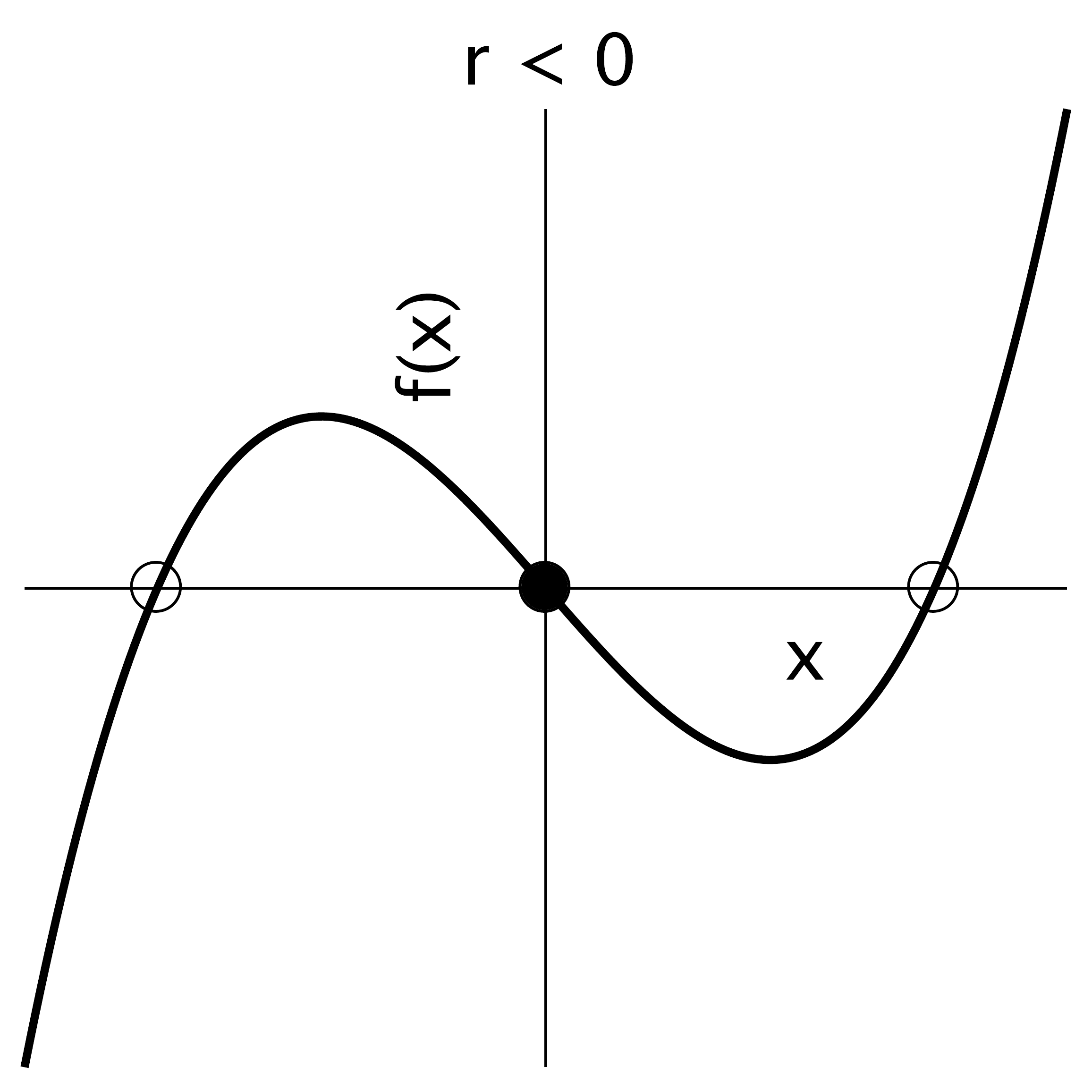
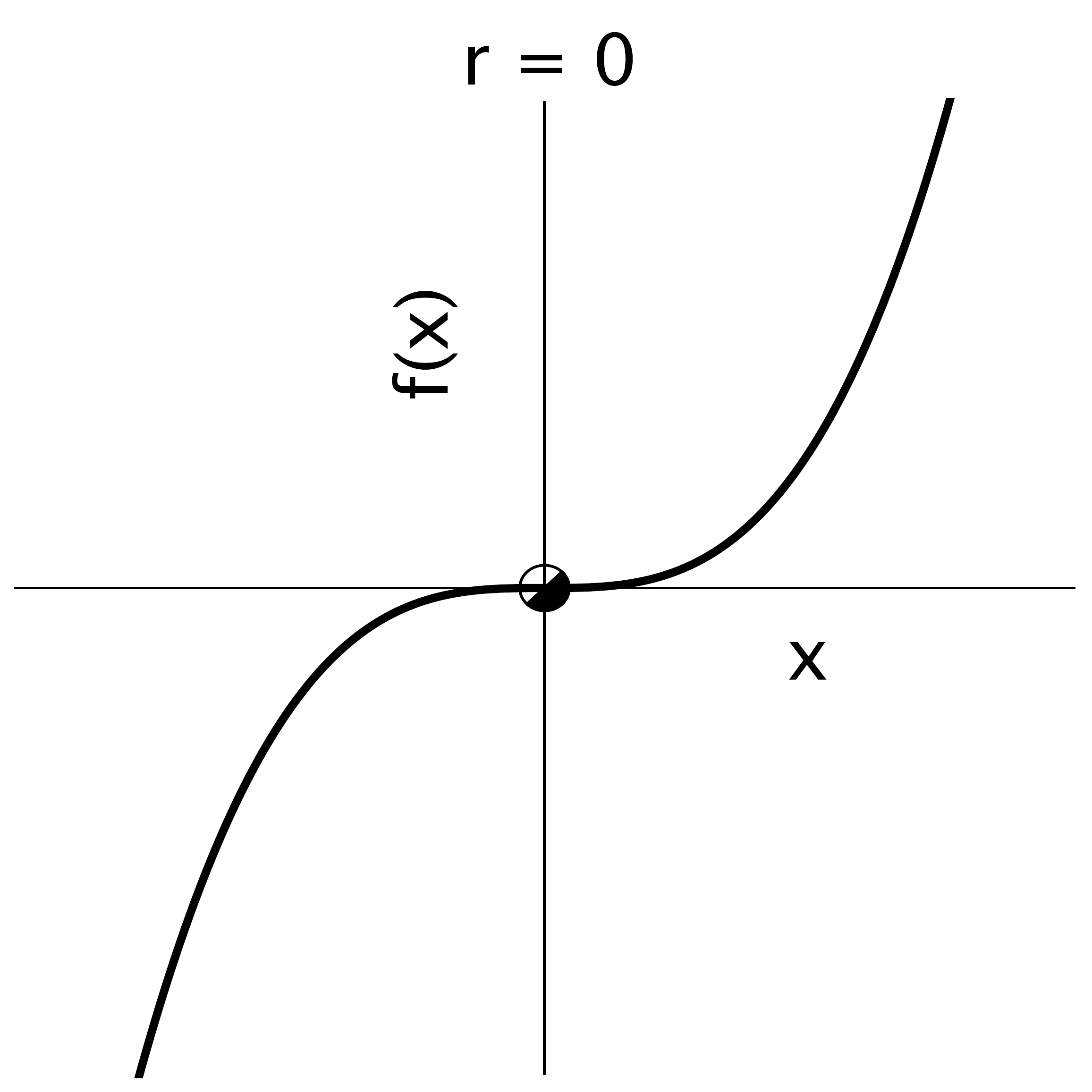
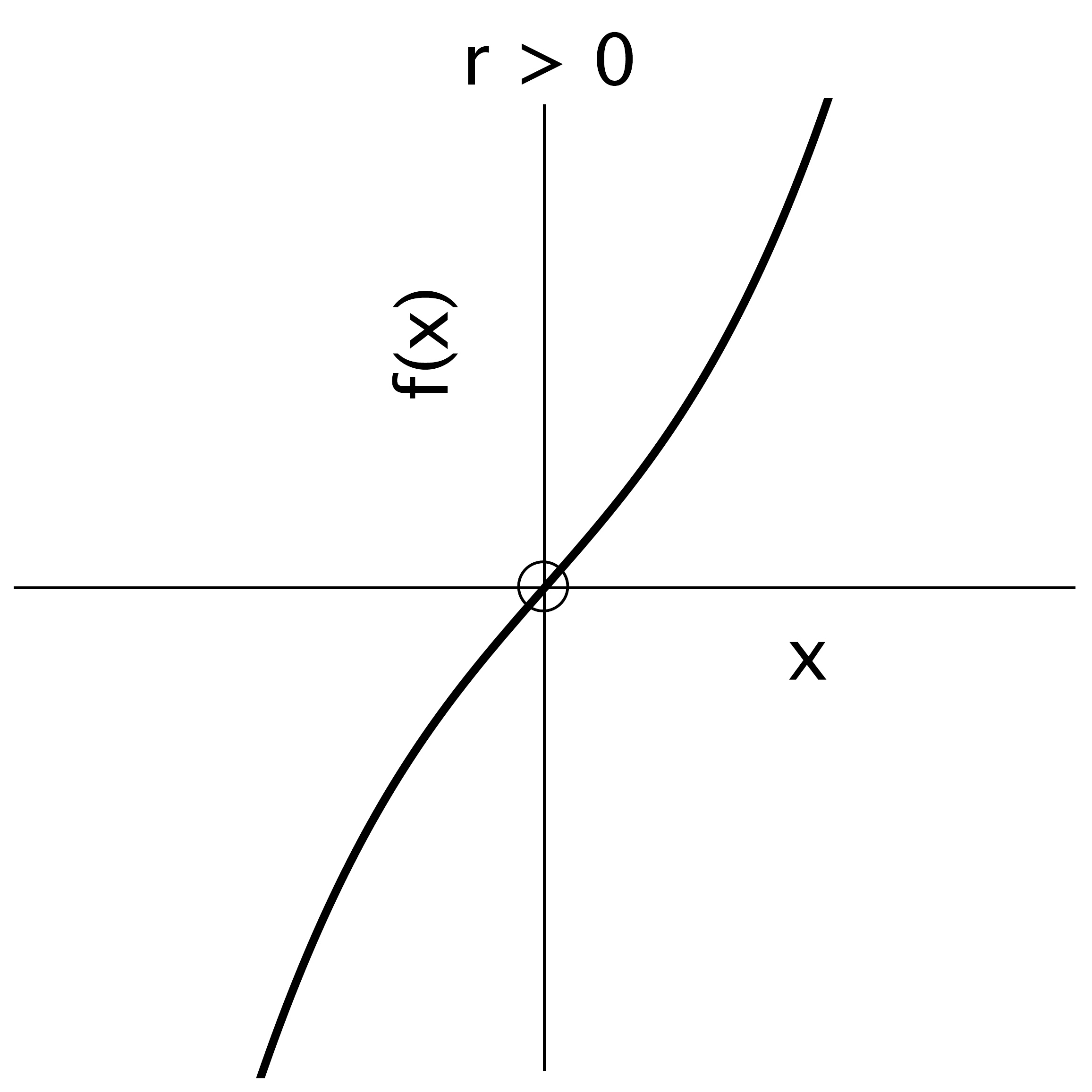
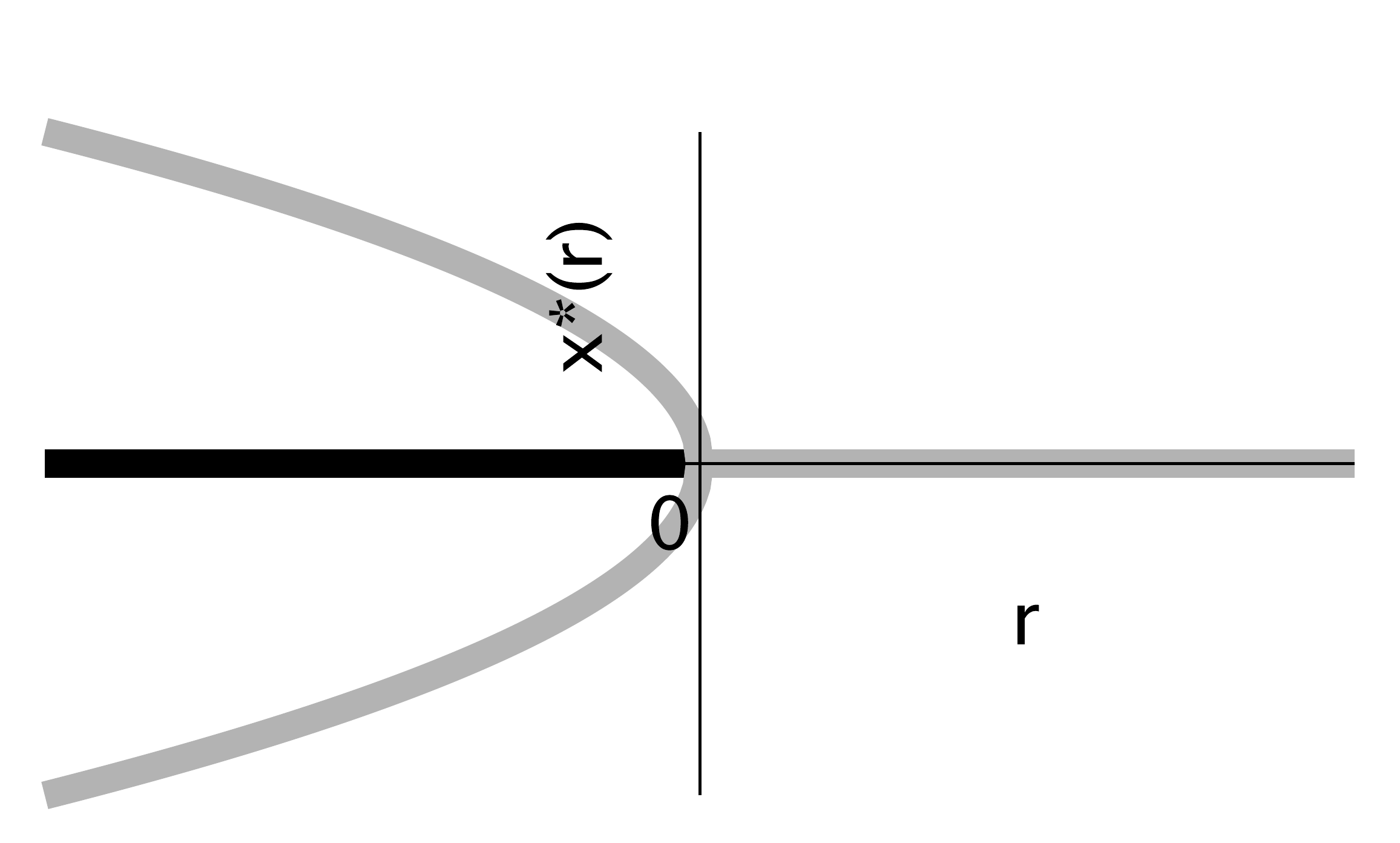
Figure 4.6 Subcritical pitchfork bifurcation in \(\dot{x} = rx+ x^3\). The bifurcation diagram in (d) corresponds to graphs (a)-(c). A black color means that the fixed point \(x_*(r)\) is stable, whereas gray means unstable. (d) Bifurcation diagram.#
4.6. Example of bifurcations: Ferromagnetic system#
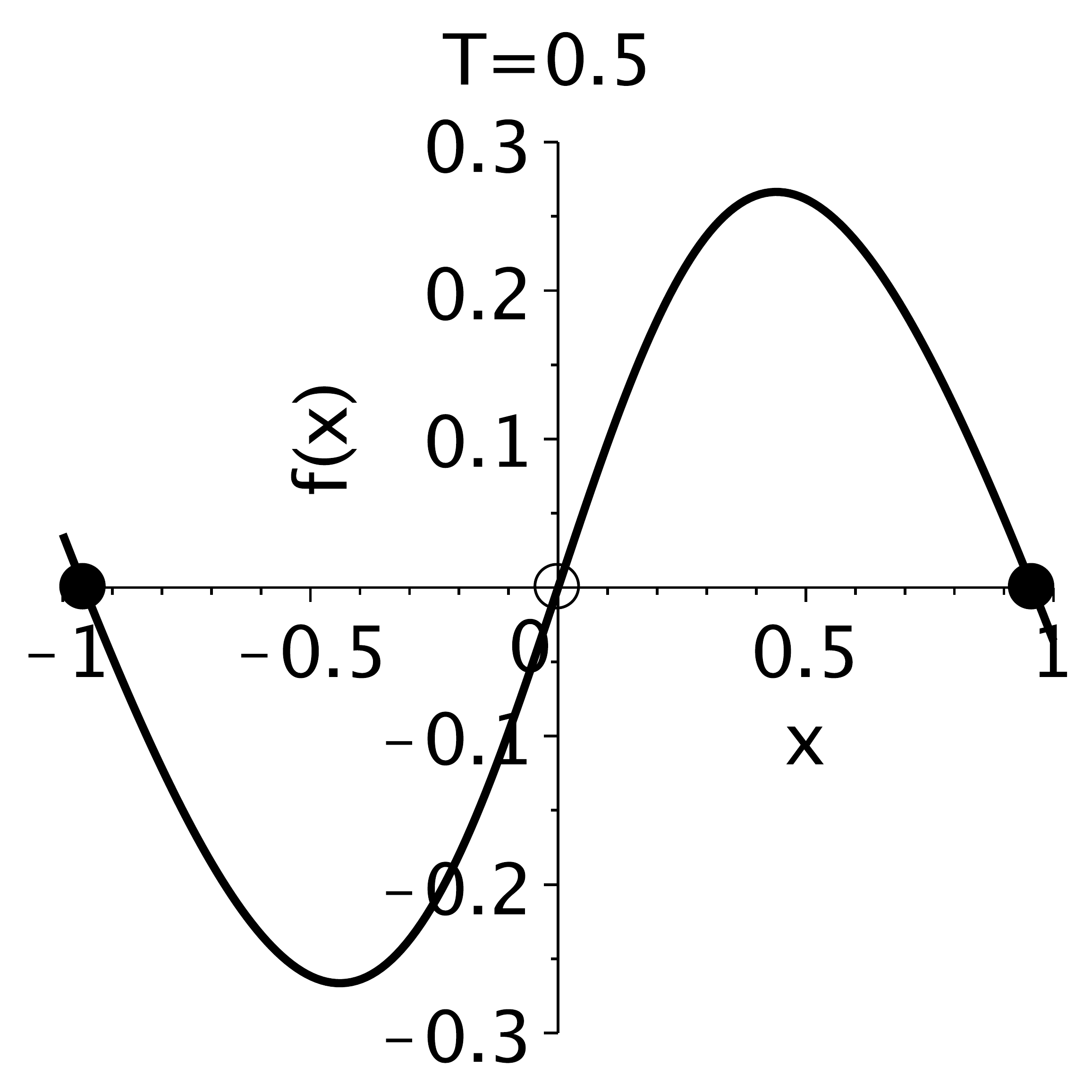
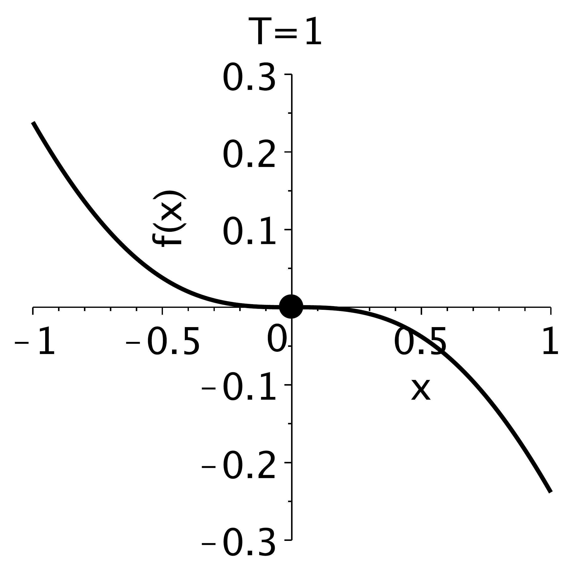
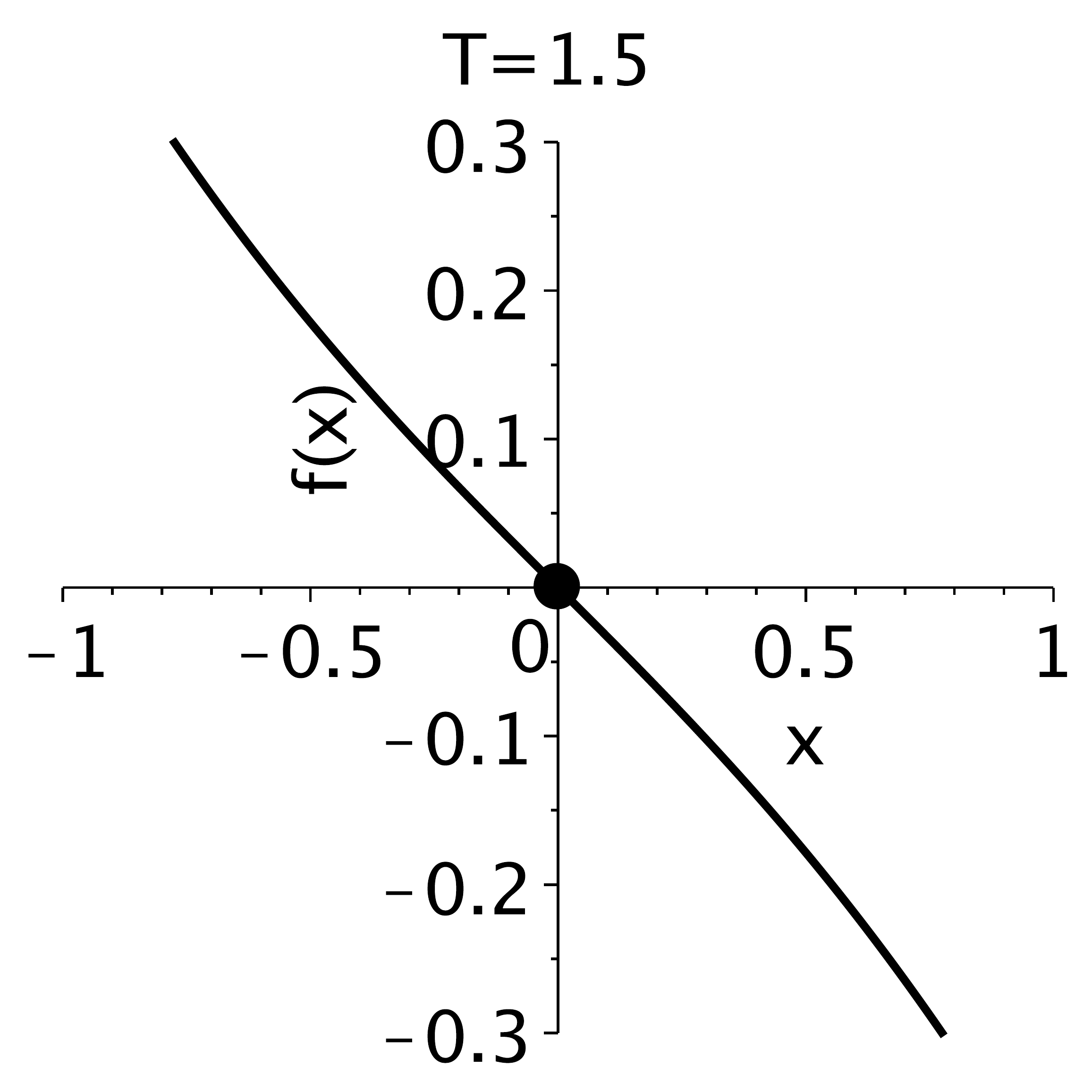
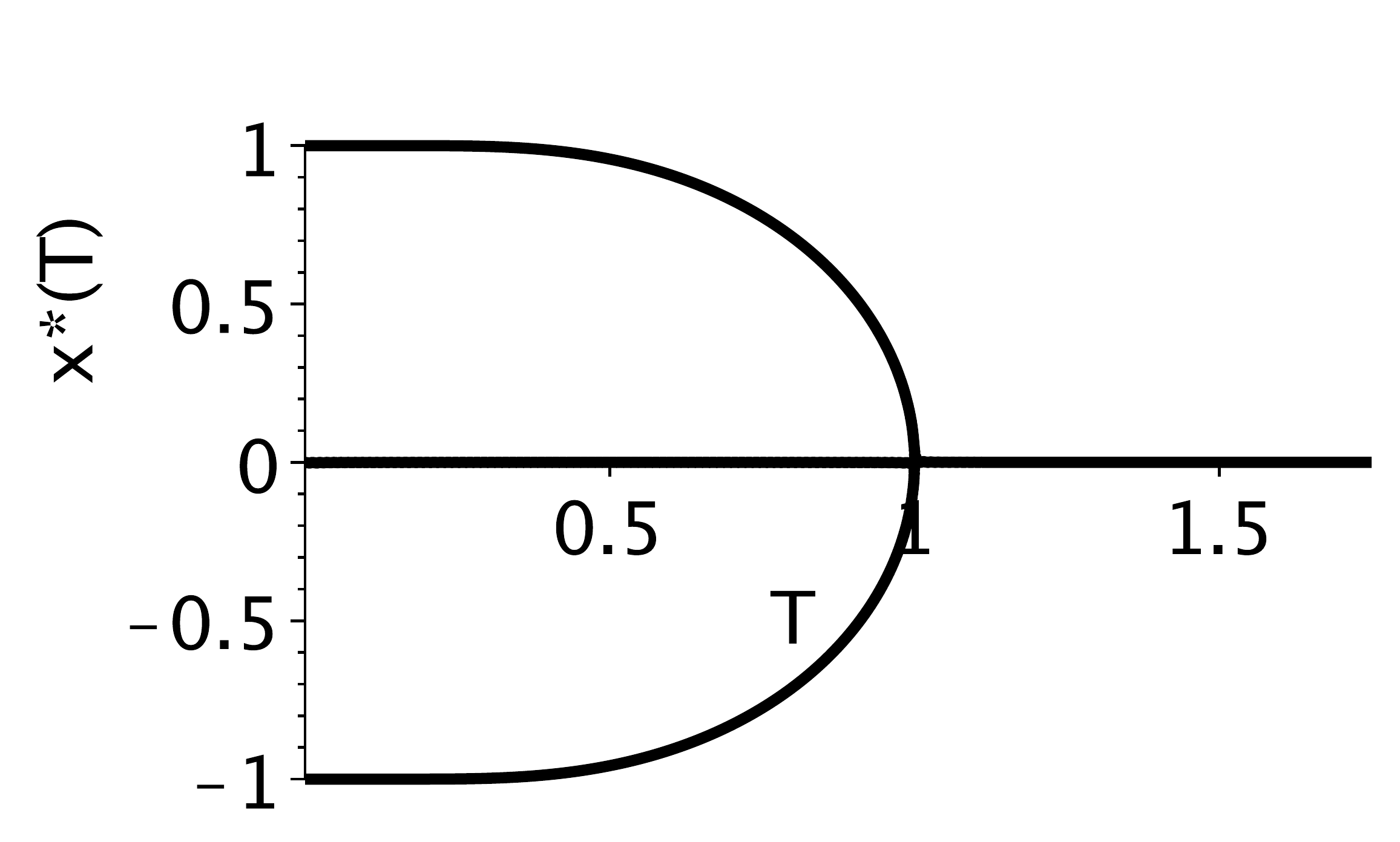
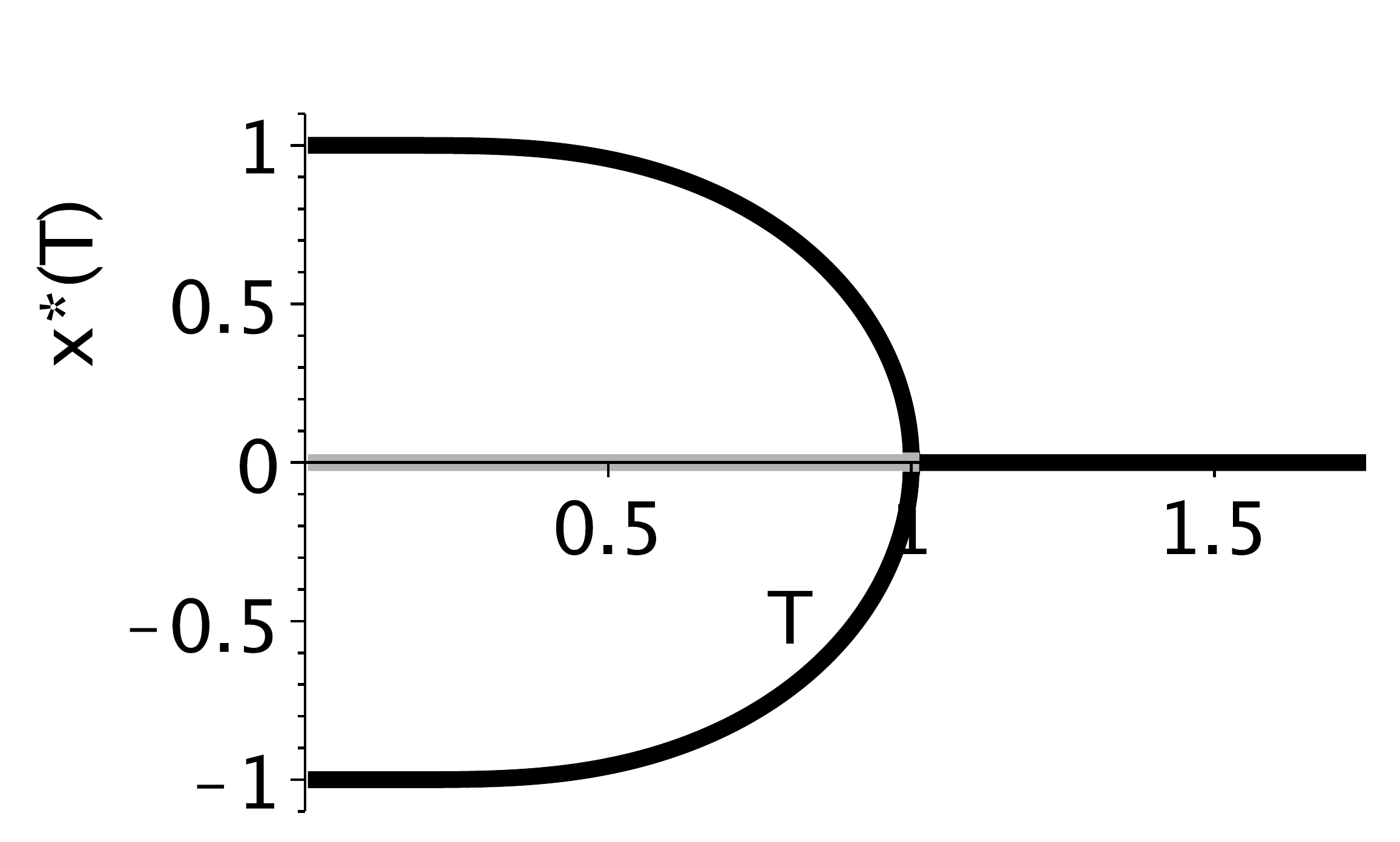
Figure 4.7 Pitchfork bifurcation in \(\dot{x} = f(x,T)=-x + \tanh\left(\frac{x}{T}\right)\). (d) Bifurcation diagram obtained by straightforwardly using implicitplot (see text). (e) Bifurcation diagram with indication of the stability of the branches.#
The governing equation for the mean magnetization \(x\) of a ferromagnetic system at (rescaled) temperature \(T\) is given by
where \(m\) represents an externally applied magnetic field. More information about this system can be found in the Infobox below. First we consider the case without external magnetic field \(m=0\). In Figure 4.7(a)-(c) we have plotted \(f(x,T)\) for various values of \(T\) which reveal three fixed points at \(0<T<1\) (two stable and one unstable), two of which are destroyed at \(T=1\) leaving one stable fixed points \(x_*(T)= 0\) for \(T\geq 1\). Such simultaneous creation/annihilation of two fixed points is characteristic of a pitchfork bifurcation. A convenient way to study the parameter dependence graphically is by using the plot command animate, see below. Figure 4.7 shows the bifurcation diagram. It is difficult to describe the branches by a simple analytical expression, since they are a solution to
so plotting a bifurcation diagram is not straightforward. But a fast way to do this is by making use of maple's implicitplot:
Maple
restart: with(plots):
f := x->-x + tanh(x/T); # define system
animate(plot,[f(x),x=-1..1],T=0.1..2.0,labels=["x","f(x)"]);
implicitplot(f(x),T=0..2,x=-1..1,gridrefine=3,labels=["T","x*(T)"]);
The implicitplot command plots the solution to \(f(x,T)=0\) within the supplied range of \(T\) and \(x\), i.e. it shows the fixed points \(x_*\) as a function of \(T\). Since there is no explicit expression, the method employs a grid to find a numerical solution. The default grid is rather coarse however, which is why we made use of the option gridrefine=3. This method using implicitplot is very powerful to get a quick glimpse of the fixed-point dependence on the external parameters (\(T\) in this case), but note that it does not provide information on the stability of the branches. Unfortunately, we have not been able to figure out a simple way in {maple } to draw the fixed point branches and color them by their stability characteristics. For lack of anything better, below we present a somewhat contrived workaround, but which seems to do the job nonetheless (see Figure 4.7)
Maple
restart: with(plots):
f := (x,T)->-x + tanh(x/T);                        # define system
df := D[1](f);                                     # derivative to x
wu := proc(T,x) f(x,T)^(-sign(df(x,T))); end proc: # unstable branch
ws := proc(T,x) f(x,T)^( sign(df(x,T))); end proc: # stable branch
implicitplot([wu,ws],0..1.75,-1..1,gridrefine=4,color=[green,red],
                                      thickness=3,signchange=false);
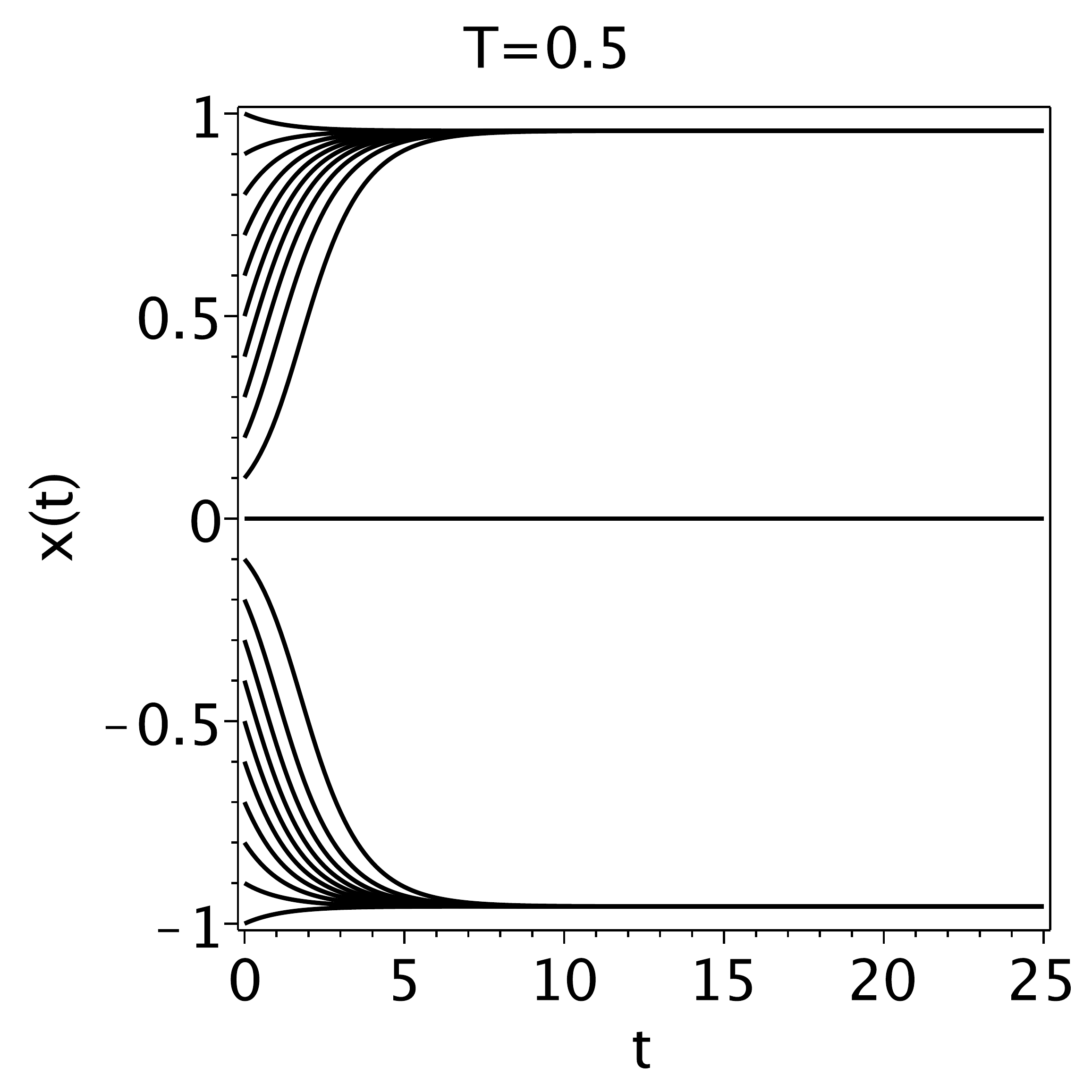
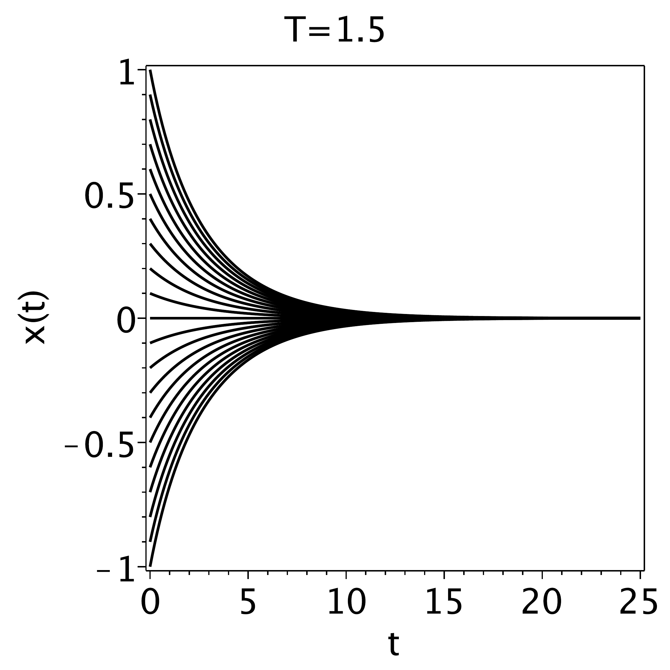
Figure 4.8 Evolution of the magnetization \(x\) for different values of the temperature \(T\). In each panel the numerical solution is shown for 20 initial conditions.#
In Figure 4.8 the numerical solution of \(x(t)\) is plotted for a number of initial conditions, and two values of \(T\). Such a figure can be made by using a loop, storing the plots and displaying them at the end:
Maple
restart; with(plots):
f := x->-x + tanh(x/T);                        # define system
eq:=diff(x(t),t)=f(x(t));                      # define differential eq
N := 20;                                       # nr of initial cond.
T := 0.8;                                      # set Temperature
for n from 0 to N do
  x0 := -1+2.0*n/N;                            # set initial condition
  sol:=dsolve({eq,x(0)=x0},x(t),type=numeric); # calculate num. solution
  P[n] := odeplot(sol,[t,x(t)],0..30):         # store the plot
end do:
display(seq(P[n],n=0..N),labels=["t","x(t)"]); # show all graphs
It is easy to verify that \(x_*= 0\) is a fixed point for all values of \(T\). The derivative of \(f(x,T)\) is
so the stability of \(x_*= 0\) is
so \(x_*=0\) is stable if \(T > 1\) and unstable if \(T<1\). The stability of the two other branches is less straightforward because we have no analytical expression for them. In the maple fragment below we calculate the numerical solution for \(T=0.5\) and evaluate the derivative to get the stability of the fixed point.
Maple
restart; with(plots):
f := x->-x + tanh(x/T);
dfdx := D(f);                             # derivative of f
T := 0.5;                                 # set T
xfp := fsolve(f(x)=0,x=0..1,avoid={x=0}); # get the non-zero fixed point
sigma := dfdx(xfp);                       # evaluate deriv. at fxd point
This yields \(x_* = 0.957\ldots, \sigma = -0.833\ldots\), showing that the fixed points is stable indeed at \(T=0.5\).
To see that the normal form of the bifurcation is \(\dot{x} = rx - x^3\), we apply a Taylor approximation around the point of bifurcation, i.e. \(T=1,x=0\). First we substitute \(q=T-1\) to translate the bifurcation to \(q=0\) which is more convenient. In maple it looks like
Maple
restart; with(plots):
f := (x,q)->-x + tanh(x/(q+1));
f_taylor := mtaylor(f(x,q),[x=0,q=0],4);
collect(f_taylor,x);
which yields
Upon substitution \(z= x/\sqrt{3}\) and \(r=q^2-q\) one obtains \(\dot{z} = rz - z^3\), which is the normal form of the pitchfork bifurcation, see Figure 4.3.
4.6.1. Non-zero external magnetic field#
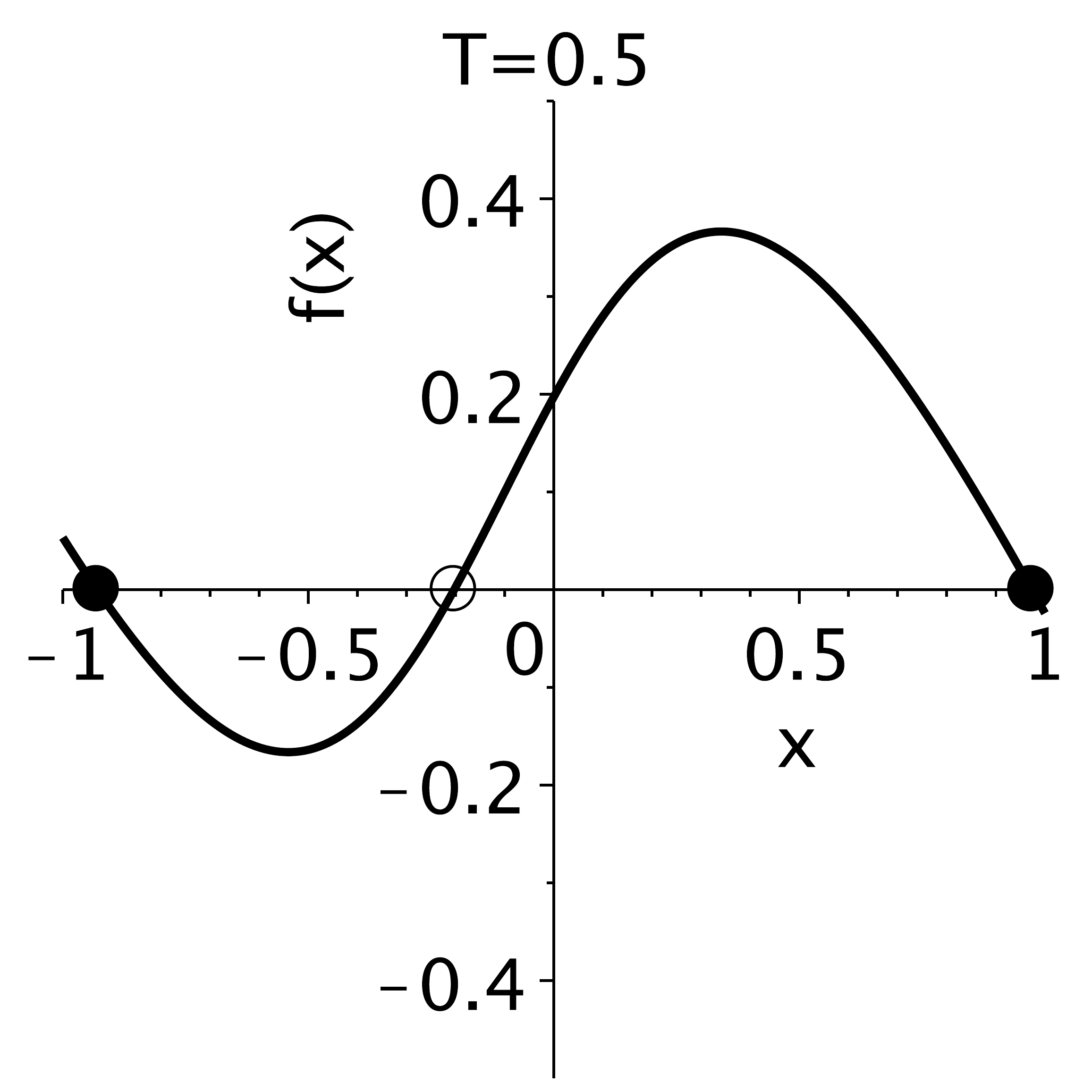
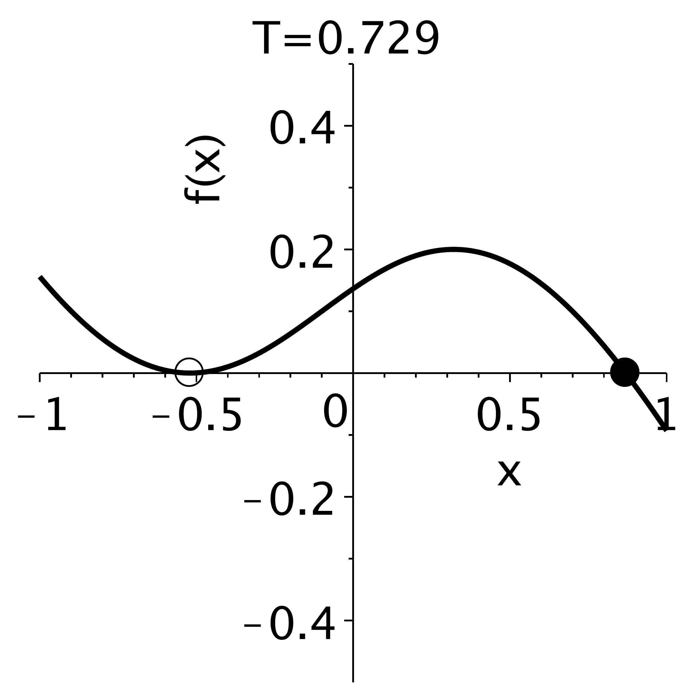
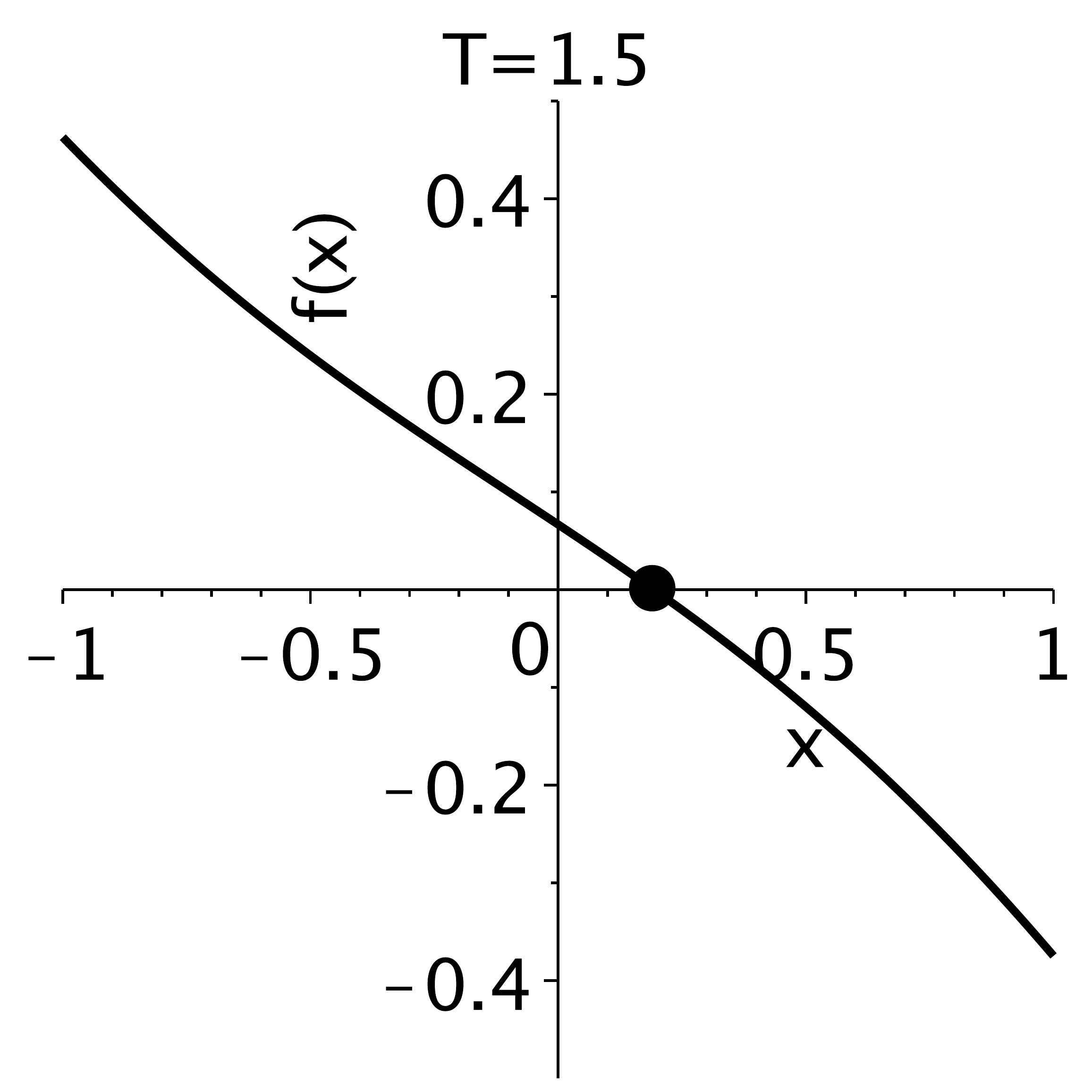
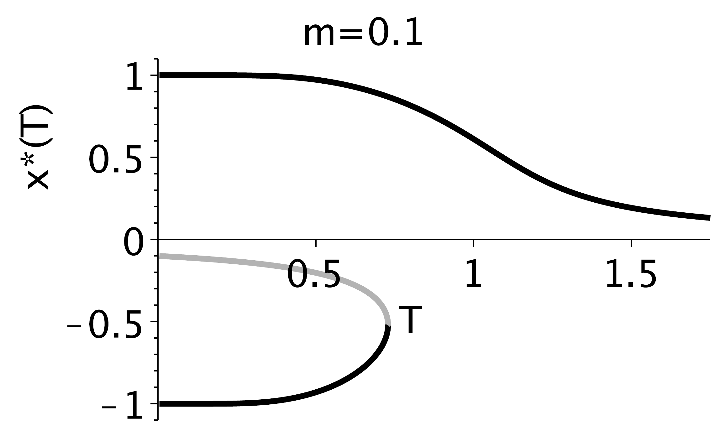
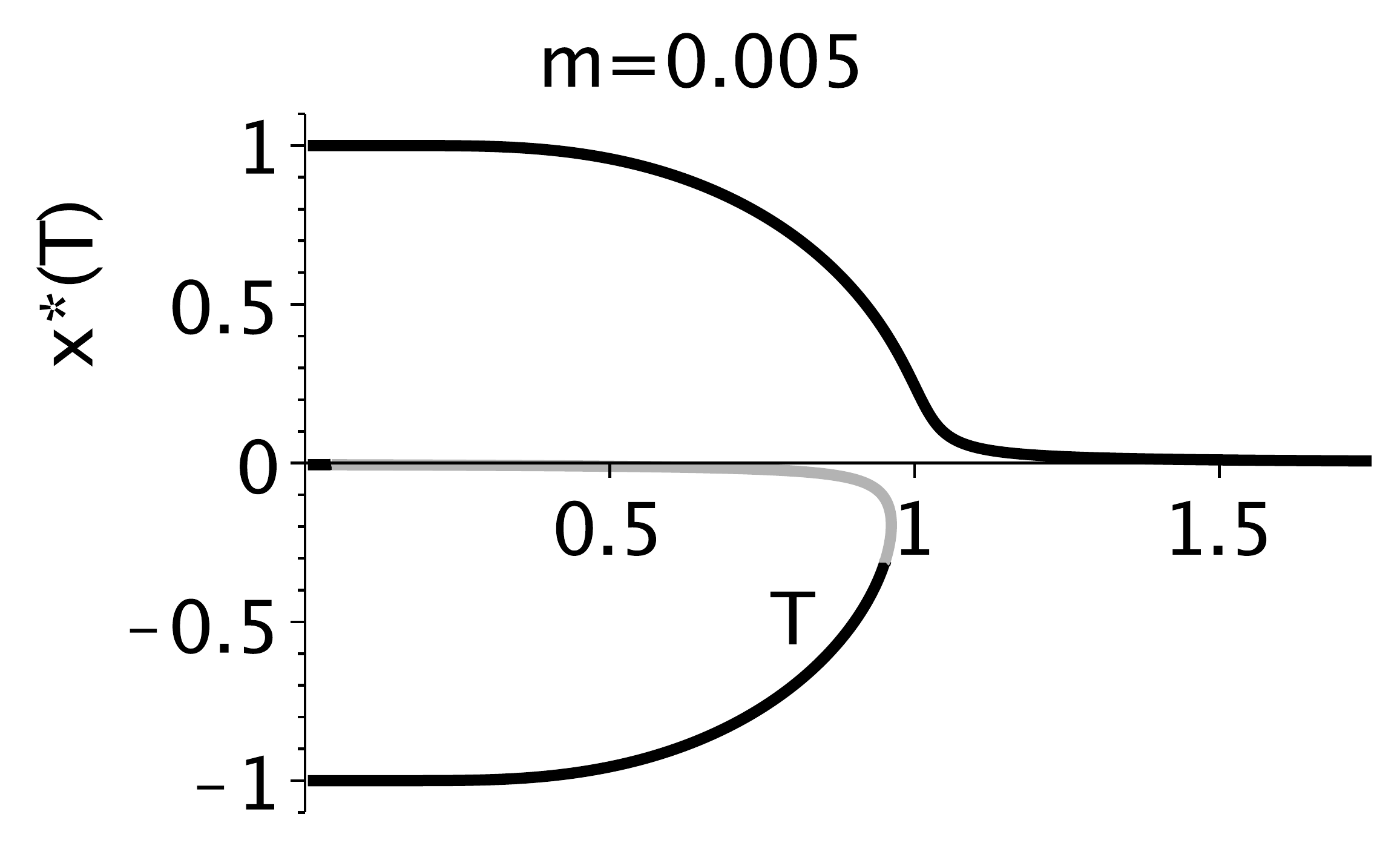
Figure 4.9 (a)-(c) Graphs of \(f(x,T)=-x + \tanh\left(\frac{x+m}{T}\right)\) for an external magnetic field of \(m=0.1\). (d) Fixed point branches \(x_*(T)\) for \(m=0.1\) and (e) for \(m=0.005\). Both cases display a saddle-node bifurcation, but as \(m\) becomes smaller, the diagram starts to more closely resemble that of a pitchfork bifurcation for \(m=0\).#
The bifurcation characteristics change substantially when a non-zero external magnetic field is applied. Let us consider \(m=0.1\). Graphs of \(f(x,T)=-x + \tanh\left(\frac{x+m}{T}\right)\) are shown in Figure 4.9. The solutions to \(f(x,T)=0\), i.e. the fixed point branches \(x_*(T)\), are shown in Figure 4.9. It was again made with implicitplot together with the abovementioned trick to get information on the stability of the branches.
It is interesting to note that the fixed point branches in this case no longer display a pitchfork bifurcation as was the case for \(m=0\) (see Fig Figure 4.7). Rather, the upper branch, \(x_*(T) >0\), is no longer involved in any bifurcation. The lower two branches, on the other hand, now display a saddle node bifurcation, compare Figure 4.4. Making a similar plot for \(m=0.005\) in Figure 4.9 shows that as \(m\rightarrow0\) the saddle node bifurcation and the upper fixed point branch will 'melt' together, such that one will retrieve a pitchfork bifurcation at \(m=0\),
To locate the critical value of \(T_c\) at which the bifurcation takes place, we search the combination of \(x_c\) and \(T_c\) that satisfy
for which we use fsolve. See maple fragment below. For \(m=0.1\) this yields for example \(T_c = 0.7287\ldots\), \(x_c = -0.520\ldots\).
Maple
restart: with(plots):
f  := x->-x + tanh((x+m)/T);              # define system
df := D(f);                               # derivative
m  := 0.1;                                # set external field
sol:=fsolve({f(x),df(x)},{x=-0.5,T=0.7}); # find (xc,Tc)
4.6.2. Example: Ferromagnetic system#
As a model of a ferromagnet we conceive of a collection of \(N\) spins \(s_i = -1,1\) (i.e. down or up), \(i=1,\ldots,N\). The spins influence each other's local magnetic field \(h\)
where the matrix coefficients \(J_{ij}\) express the connection strength between spin \(i\) and spin \(j\); \(m\) represents an externally applied magnetic field (if any). One could for example account for the distance between the spatial location \(\mathbf{z}_i\) of the spins by taking \(J_{ij} = f(|\mathbf{z}_i-\mathbf{z}_i|)\), but here we study the simplified situation where all connections are equal \(J_{ij} =1\).
The state of the system at time instance \(t\) is given by the vector \(\mathbf{s}\). Given that each spins can attain one of two possible states, there are \(2^N\) possibilities for \(\mathbf{s}\). If the systems has temperature \(T\), the probability of a particular state \(\mathbf{s}\) is given by the Boltmann distribution
where \(H(\mathbf{s})\) is the Hamiltonian \(H(\mathbf{s}) = \frac{1}{2} \sum_{ij} s_i J_{ij} s_j\).
One can simulate the ferromagnet by 1) randomly picking a spin from the ensemble, say number \(i\), 2) calculating the local field \(h_i\) by (4.12), and 3) flipping its state \(s_{i} \rightarrow -s_{i}\) with probability \(p(s_{i} \rightarrow -s_{i}) \sim \exp(-s_i h_i/T)\). One can prove that the distribution of states given by (4.13) will be satisfied if the transition probability is chosen as
In the limit \(T\rightarrow 0\) this implies that if \(s_i\) is not aligned with its local field \(h_i\), that is \(h_i<0\) while \(s_i = +1\) or \(h_i > 0\) while \(s_i = -1\), then the probability of flipping \(s_i\) limits to 1, such that the spins will get aligned to the local field: \(s_i \rightarrow \text{sign}(h_i)\). For \(T>0\), however, there is a non-zero probability that \(s_i\) and \(h_i\) remain disaligned.
The following maple program gives an implemtation that simulates a ferromagnetic system at predefined temperature \(T\). In Figure 4.10 we give an example of the evolution of \(N=400\) spins from two different initial states for \(T=0.5\) and \(T=1.5\). The external magnetic field was set to \(m=0\). The initial state (see also the maple code) is created by setting all spins to \(+1\) and flipping a preset fraction \(F\) of them.
Maple
restart; with(plots):
K := 20;
N := K*K;                   # number of spins
show_state := proc(s)       # show the current state
local i,j;
global K;
  listdensityplot([seq([seq(s[j+K*(i-1)],i=1..K)],j=1..K)],range=-1..1);
end proc:
choose_spin := 1 + rand(N): # choose spin at random
R := 10000:
random := evalf(rand(R)/R): # draw rnd nr from [0..1>

s  := Array(1..N,1):        # define spins and set to +1
F := 0.2;
for i from 1 to N do
  if( random() < F ) then   # flip or not
     s[i] := -s[i];
  end if;
end do:
show_state(s);

m := 0;                     # set external field
T := 0.5;                   # set Temperature
iter := 10000;              # set number of iterations

nrplots := 0;
for n from 0 to iter do     # dynamics

  i := choose_spin();
  h_i := evalf(add(s[j],j=1..N)/N + m);          # calc local field
  F := evalf((1 + tanh(s[i]*h_i/T))/2.0);        # calc transition prob
  if( random() > F ) then s[i] := -s[i]; end if; # flip spin or not

  if( n mod 200 = 0 ) then
    nrplots := nrplots + 1;
    pl[nrplots] := show_state(s);                # store some plots
  end if;

  x[n] := evalf(add(s[j],j=1..N)/N);             # store mean state

end do:
# click in window to animate evolution of spins ...
display(seq(pl[k],k=1..nrplots),insequence=true);
# show mean state in time
plot([seq([n/N,x[n]],n=0..iter)],view=[0..iter/N,-1..1],labels=["t","x(t)"]);

Figure 4.10 Evolution of the spin dynamics from two different initial states for two temperatures. The corresponding mean states are displayed in Figure 4.11.#
To give a macroscopic description of the system, it is useful to calculate at each instance the mean magnetization of the spin system
which yields a value \(\in [-1,1]\). In the limit \(N\rightarrow \infty\) one can derive that the dynamics of \(x(t)\) is given by
In Figure 4.11 we display the evolution of \(x\) for the cases corresponding to Figure 4.10. Apart from so-called finite size fluctuations (i.e. \(N\) is not large enough), the evolution resembles that of Figure 4.8 reasonably well. An even better match will be obtained when the number of spins \(N\) is further increased.
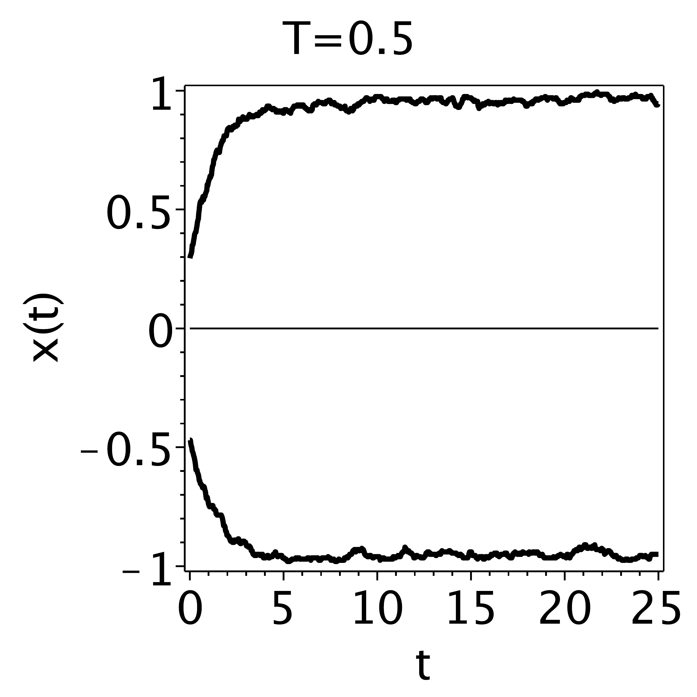
Figure 4.11 Evolution of the mean state \(x\) as a function of time \(t=n/N\) for the cases shown in Figure 4.10. Compare also with Figure 4.8.#
4.7. Catastrophes, hysteresis, and phase transitions#
A saddle node bifurcation is sometimes also called 'hard bifurcation', as opposed to transcritical and pitchfork bifurcations which are called 'soft bifurcation'. The reason for these terms can be understood by looking for instance at the saddle node bifurcation in figure Figure 4.9. If one starts at \(T=0\) at the lower branch (\(x_*\simeq-1\)) and one increases \(T\) in a slow manner such that the dynamical system has sufficient time to converge to the fixed point that belongs to the new temperature, one will move along the branch to the right. This can continue until \(T_c = 0.7287\ldots\) has been reached. Here the fixed point value is \(x_* = x_c = -0.520\ldots\). After a tiny increase of \(T\) beyond \(T_c\), there is no longer a fixed point in the vicinity, so the system will rapidly move to the upper fixed point branch. Usually this is a dramatic event for the system, sometimes referred to as 'catastrophe', which explains the name 'hard bifurcation'. In a pitchfork or transcritical bifurcation there is no need for a 'jump' to another branch because a smooth ('soft') transition to another branch is possible. Physicist tend to use the terms 'first order phase transition' and 'second order phase transition' for hard and soft bifurcations, respectively.
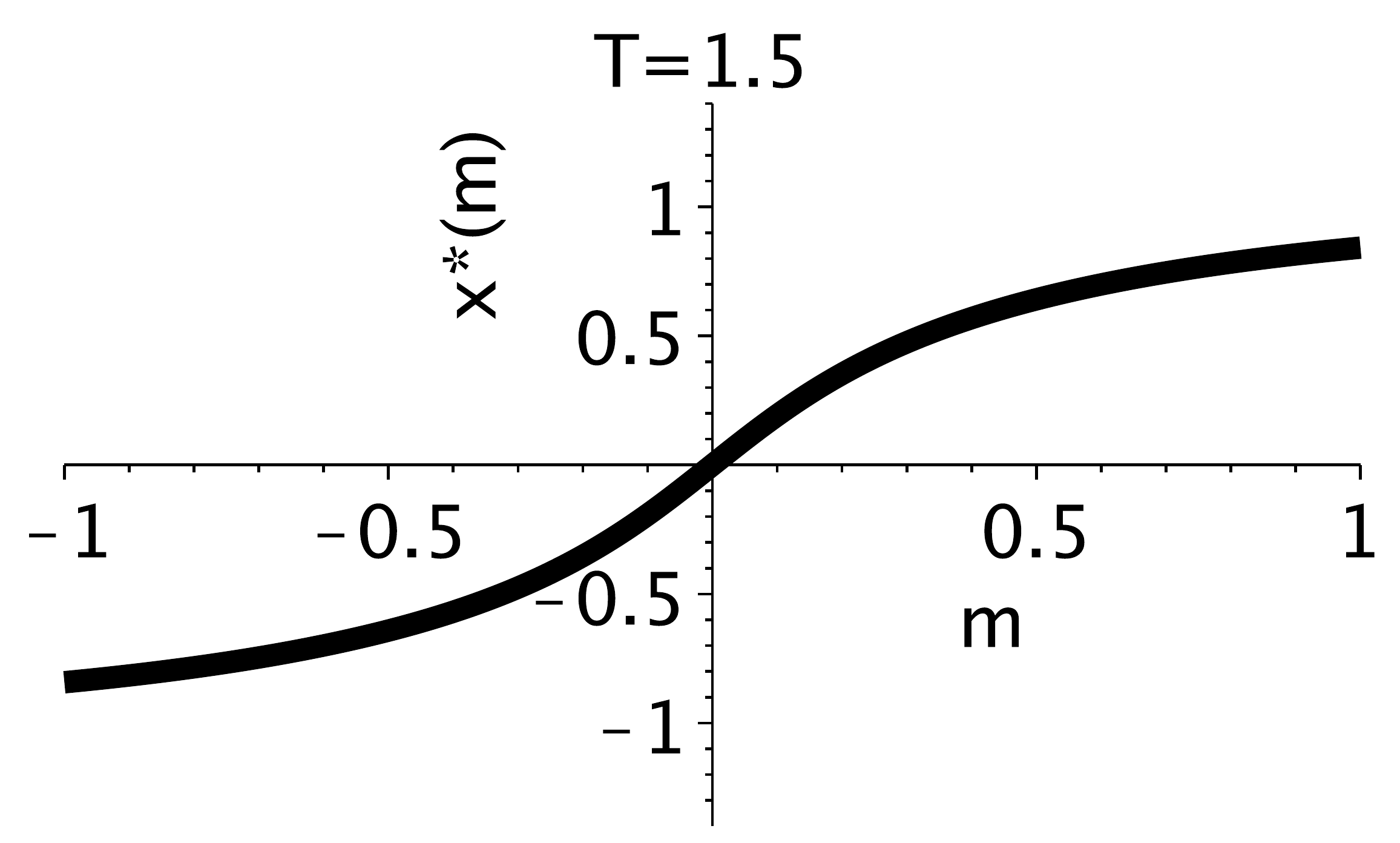
Figure 4.12 Left column: Fixed point braches as a function of the external magnetic field \(m\) for different values of the temperature \(T\). The branches were determined using implicitplot. Unstable branches are colored gray. Right column: Fixed points determined by numerical integration of the governing equation \(\dot{x}=-x+\tanh[(x+m)/T]\) each step using the previously computed fixed point as initial condition. In each of these panels first a forward sweep \(m=-1..+1\) is conducted, followed by a backward sweep \(m=+1..-1\). The plots illustrate the hysteresis effect when \(T<1\), together with the occurence of 'hard' bifurcations as demonstrated by the suddden jumps to the other branch.#
Let us reconsider the ferromagnetic system, but now use \(m\) as the bifurcation parameter instead of \(T\). Using implicitplot we have plotted in the left column of Figure 4.12 the fixed-point branches as a function of \(m\) for various values of \(T\). The branches for \(T\geq 1\) appear not to be involved in any bifurcation. But the branches for \(T<1\) are much more interesting: as the branches seem to get 'folded', they exhibit two saddle node bifurcations. Apart from plotting these branches with implicitplot, it is illustrative to show the actual behaviour of the system by numerically integrating the system and computing its steady state point. These graphs are plotted in the right column of Figure 4.12. We have used the following maple code to obtain these plots.
Maple
restart; with(plots):
f := (x,m)->-x + tanh((x+m)/T);
eq:=diff(x(t),t)=f(x(t),m);
T := 0.5; mmin := -1.0; mmax :=  1.0;
N := 200;
tinf := 100;                     # long time
ic := x(0) = -1;
for n from 0 to N do             # forward sweep from h = -1 to +1
  m := mmin + n*(mmax-mmin)/N:
  sol:=dsolve({eq,ic},x(t),type=numeric):
  X1[n] := subs(sol(tinf),x(t)); # large time solution
  M1[n] := m;
  ic := x(0) = X1[n];            # use previous value as initial cond.
od:
for n from 0 to N do             # backward sweep from h = +1 to -1
  m := mmax - n*(mmax-mmin)/N:
  sol:=dsolve({eq,ic},x(t),type=numeric):
  X2[n] := subs(sol(tinf),x(t)); # large time solution
  M2[n] := m;
  ic := x(0) = X2[n];            # use previous value as initial cond.
od:
p1 := plot([seq([M1[n],X1[n]],n=0..N)]): # plot forward sweep
p2 := plot([seq([M2[n],X2[n]],n=0..N)]): # plot backward sweep
display(p1,p2,view=[-1..1,-1.4..1.4],labels=["m","x*"]);
Note that we perform two sweeps. First we increase \(m\) from \(-1\) to \(1\) in small steps and calculate at every step the 'large time' solution (\(t=100\) in this case). As initial condition we take the final value of \(x\) calculated in the previous step. In the second sweep the direction of \(m\) is reversed (\(+1\rightarrow -1\)). The plots in the right column of Figure 4.12 nicely reveal two aspects of the system. Firstly, the sudden jumps, or 'catastrophes', that occur when \(T<1\), demonstrating the 'hard bifurcations' in the system. Secondly, one can notice hysteresis: the forward sweep is different from the backward sweep. By integrating the system one cannot show the location of the unstable braches, such as in the left column. On the other hand, it provides a good view of how the system really responds. Figure 4.13 combines the plots of the left column and right column of Figure 4.12 for the case of \(T=0.5\), illustrating the stable and unstable parts of the branch, the jumping from one branch to the other (hard bifurcations), and the hysteresis in the system. The right panel shows a three-dimensional view, illustrating the 'folding' of the fixed-point manifold that causes the saddle node bifurcations. The plot, including the shading, was made using one call to implicitplot3d:
Maple
restart; with(plots):
implicitplot3d(-x + tanh((x+m)/T),x=-1..1,T=0.5..1.5,m=-1.1..1.1,
           view=[-2..2,0.5..1.5,-1.4..1.4],
           grid=[50,50,50],style=surface,orientation=[-165,8,-122],
           style=surface,color=gray,light=[45,20,0.8,0.8,0.8]);
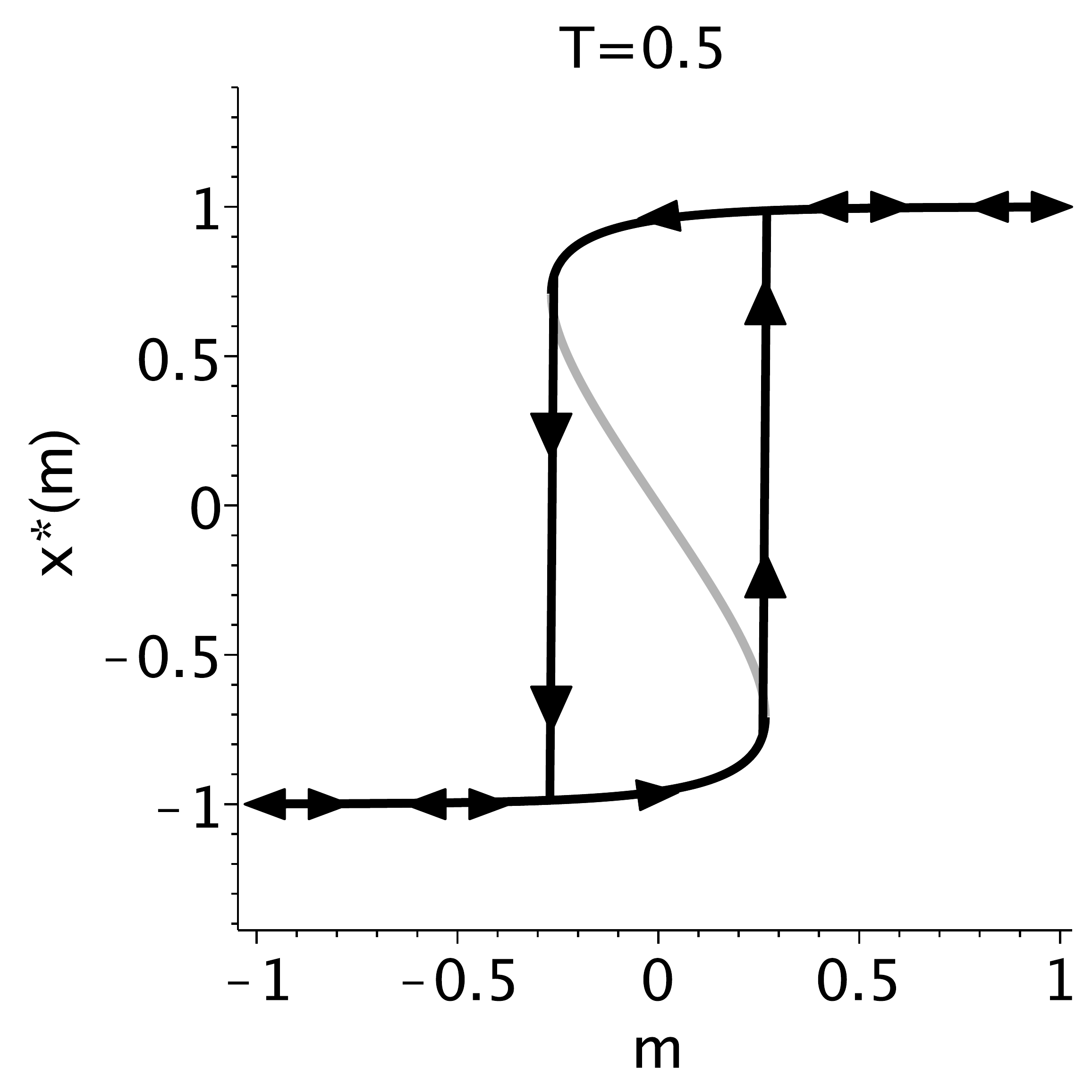
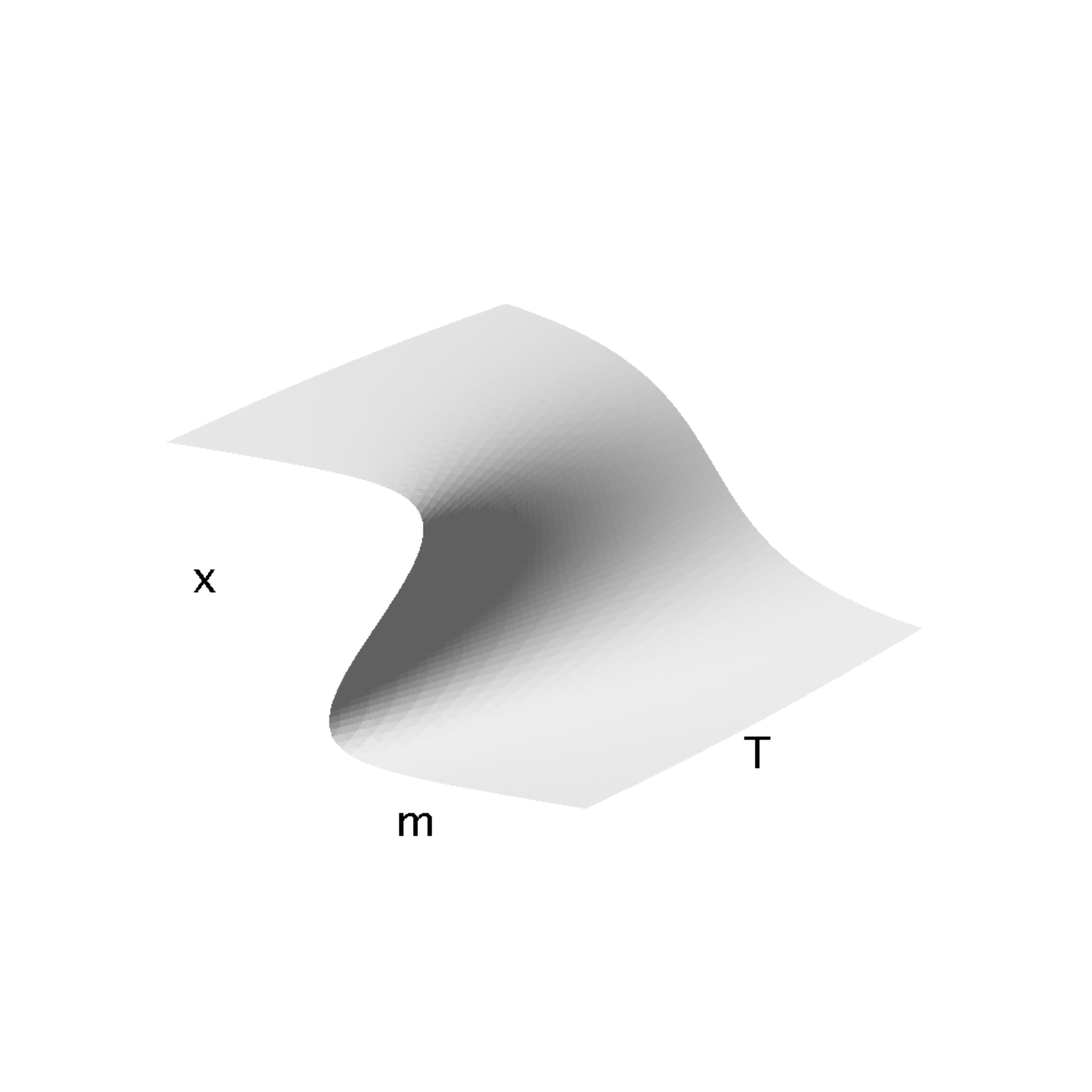
Figure 4.13 (a) Hysteresis and hard bifurcations in the ferromagnetic system with external field \(m\). (b) 'Folding' of the fixed point manifold.#
4.7.1. Example: multiple equilibria in the climate system#
The earth's average temperature results from a balance between \(Q_{\text{in}}\), the short-wave radiation received from the sun, and a loss \(Q_{\text{out}}\) due to long-wave radiation emitted by the earth. If \(R\) is the radius of the earth and \(\pi R^2\) the area of the disk that is illuminated by the sun, the energy input to the earth per unit time is \(Q_{\text{in}} = \pi R^2 S (1-a)\), where \(S=1370\) W/m \(^2\) is the solar constant and \(a\) is the albedo of the earth, i.e. the reflection coefficient in the short-wave range. Due to the energy input the earth heats up and emits (long-wave) radiation along its entire surface: \(Q_{\text{out}} = 4 \pi R^2 \epsilon \sigma T^4\), where \(T\) is the temperature \(T\) of the earth in Kelvin, and \(\sigma = 5.67\cdot10^{-8}\) kg s \(^{-3}\) K \(^{-4}\) denotes the constant of Stefan-Boltzmann. \(\epsilon\) is the effective emissivity; for black body radiation \(\epsilon = 1\), but here a 'gray body' approximation (\(\epsilon < 1\)) is more appropriate because of the presence of greenhouse gases in the atmosphere like CO \(_{2}\) and water vapour, which absorb part of the long wave radiation and hence reduce the emission of radiation. The stationary mean temperature follows from the balance \(Q_{\text{in}}=Q_{\text{out}}\).
If we account for the heat capacity of a surface layer with thickness \(h\) and specific heat \(c_v\), we arrive at the following simple dynamical model
where \(\rho\) represents the density. Dividing by \(4 \pi R^2\) and defining \(\beta = h \rho c_v\) gives
Setting \(\mathrm{d} T/\mathrm{d} t\) to zero and solving for \(T\) one obtains the stationary temperature (fixed point)
With an average albedo of \(a=0.3\) and an emissivity of \(\epsilon = 0.61\), one finds \(T^*\simeq 289\) K, close to the current global average temperature. This simple model shows the effect of increased emissions of greenhouse gases as this lowers \(\epsilon\) and hence increases the value of \(T^*\); see figure Figure 4.14. Note that the value of the parameters, i.e. \(a,\epsilon\) and \(S\) uniquely determine the stationary state \(T^*\) (there is only one possible equilibrium). This is a stable equilibrium since the derivative in the fixed point \(T_*\) is negative
Below a maple implementation
Maple
restart: with(plots):
f := T -> ((1-a)*S/4-epsilon*sigma*T**4)/beta;
sigma := 5.67e-8; beta := 4e7; S := 1370;
a := 0.3; epsilon := 0.61;
# fixed point
Teq := fsolve(f(T)=0,T=0..350);
# stability, determine the derivative in the fixed point
df := D(f);
df(Teq);
# fixed point as a function of emissivity
epsilon := 'epsilon';
implicitplot(f(T),epsilon=0.3..1,T=100..400,gridrefine=3,labels=["epsilon","T*"]);
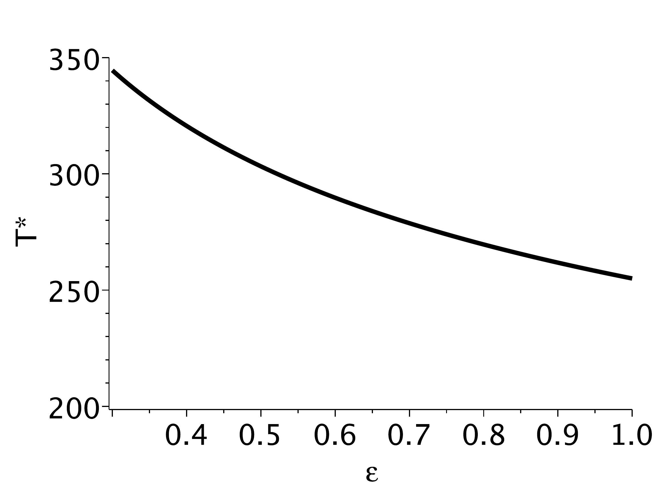
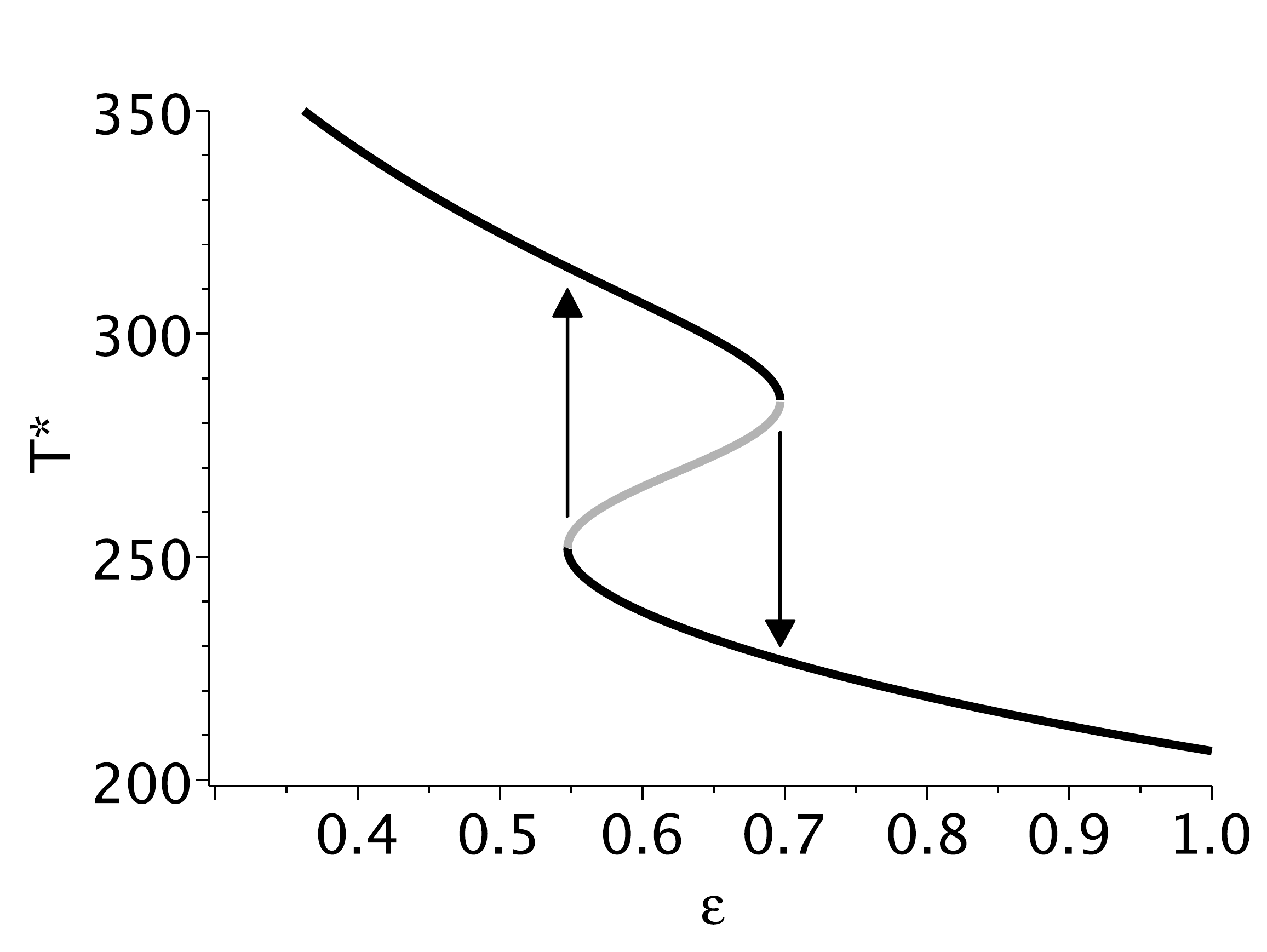
Figure 4.14 Average stationary temperature \(T_*\) of the earth as a function of the emissivity \(\epsilon\). Stable branches are black; unstable branches are gray. (a) Constant albedo \(a=0.3\). (b) Temperature dependent albedo.#
Multiple equilibria can occur when the so-called albedo feedback is taken into account. This involves an interesting dependence of the albedo \(a\) on temperature, because ice tends to reflect the incoming sunlight much more than ocean water does. This yields a positive feedback: when it is globally cold, ice sheets will prevail and much of the solar energy will be reflected, thus sustaining the cold climate. However, in a warm climate ocean water will prevail and much of the energy is absorbed, thus sustaining the warm climate. This is called the albedo-feedback, and as we will see below, it forms the reason for the existence of multiple equilibria.
To account for the temperature dependence of the albedo, we take the following simple model
where \(T_{\text{m}}\) is the melting point of ice. By virtue of the \(\tanh\) function and the value of \(\Delta T\), the albedo is a smooth function of temperature encompassing both the ice (\(T<T_{\text{m}}\)) and the liquid water state (\(T>T_{\text{m}}\)). For \(T \ll T_{\text{m}}: a=0.7\), whereas for \(T \gg T_{\text{m}}: a=0.1\). Inserting this albedo function in (4.16) and solving (numerically) for the fixed point(s) \(T_*\) reveals that for a range of \(\epsilon\) multiple equilibria occur, see Figure 4.14. One also notes the unstable branch (gray color) and the possibility for hysteresis: if one gradually increases \(\epsilon\) beyond \(0.697\), one drops to the lower (cold) branch. If one subsequently reduces \(\epsilon\) one will stays on the lower branch until the critical value \(\epsilon = 0.547\) is reached, beyond which the system jumps back to the upper (hot) branch.
The following maple fragment shows how the plot in Figure 4.14 was made and how the critical values for \(\epsilon\) were determined. For additional coloring of the branches by their stability, one can use the example given in section 4.6.
Maple
restart: with(plots):
f := T -> ((1-a(T))*S/4-epsilon*sigma*T^4)/beta;
a := T -> 0.4 - 0.3*tanh((T-Tm)/DT);
sigma := 5.67e-8; beta := 4e7; S := 1370;
Tm := 273; DT := 20;
implicitplot(f(T),epsilon=0.3..1,T=100..400,gridrefine=3,labels=['epsilon',"T*"]);
# determine the critical values of epsilon
df := D(f):
fsolve({f(T)=0,df(T)=0},{T=280,epsilon=0.6});
fsolve({f(T)=0,df(T)=0},{T=250,epsilon=0.4});
symbol |
value |
unit |
|---|---|---|
\(S\) |
1370 |
W/m\(^2\) |
\(\sigma\) |
\(5.67\cdot10^{-8}\) |
kg s\(^{-3}\)K\(^{-4}\) |
\(\epsilon\) |
0.61 |
- |
\(c_v\) |
4000 |
JK\(^{-1}\)kg\(^{-1}\) |
\(\rho\) |
1000 |
kg m\(^{-3}\) |
\(h\) |
10 |
m |
\(\beta = h \rho c_v\) |
\(4\cdot10^{7}\) |
Jm\(^{-2}\)K\(^{-1}\) |
\(T_{\text{m}}\) |
273 |
K |
\(\Delta T\) |
20 |
K |
4.8. Exercises#
4.8.1. Hysteresis#
Downloads: Hysteresis.mws
Study the equation
where \(r\) is a parameter of the system. The system undergoes a subcritical bifurcation.
Analytical approach:
a) Find an expression for the fixed points \(x^{\star}\) for arbitrary \(r\).
b) Plot \(x^{\star}(r)\) as a function of \(r\) and give each branch a different color.
c) Determine the stability of the branches.
Numerical approach:
d) Take \(r=0.3\) and \(x(0) = 0.1\); determine the numerical solution and plot the evolution of the system. Repeat this for \(r=-0.1\).
e) Create a bifurcation diagram by plotting the numerically computed 'large time solutions' as a function of \(r \in [-0.5,0.5]\) Increase \(r\) in small steps, calculate the corresponding 'large time solutions', and take as the initial conditions the equilibrium solution of the previous(!) step. In this way you simulate a slow change of the parameter \(r\): the system has time to equilibrate to the fixed points belonging to the new value of \(r\).
f) Repeat the procedure of (e) for \(r\) decreasing from 0.5 to -0.5.
g) Plot the results of (e) and (f) in the same graph, and give an explanation. You may want to include the branches obtained in (b) in the same plot.
4.8.2. Stability and bifurcations#
Downloads: PitchforkBifurcation.mws
Consider the system
with \(\nu \leq 1/2\) a parameter.
a) Find the fixed points.
b) Classify the stability of each fixed points in terms of \(\nu\).
c) Does the system exhibit a bifurcation? If so, indicate for which value of \(\nu\), classify the kind of bifurcation, and plot a bifurcation diagram.
d) Set \(\nu = 1/4\) and determine with Maple the numerical solution for the initial conditions \(x(0) = 10^{-4}\) and \(x(0) = 3\) and plot the time evolution.
4.8.3. Stability and bifurcations (2)#
Downloads: StabilityBifurcationsExp.mws
Consider the system
for \(r\in [-10,10]\).
a) Find (numerically) all fixed points for \(r=3\),
b) and classify their stability.
c) Specify the attraction domains of each these fixed points.
d) Plot \(f_{r}(x)\) for different values of \(r\) and determine from the plots how many bifurcations the system undergoes within the range \(r\in [-10,10]\)? Give a qualitative characterisation the type of bifurcations (saddle-node, transcritical, etc).
e) Prove analytically that the system undergoes a bifurcation when the stable fixed-points have the values \(x_{1}^{*} =-1 - \sqrt{2}/2\), or \(x_{2}^{*}=-1+\sqrt{2}/2\). Calculate the critical values \(r_1\) and \(r_2\) corresponding to the bifurcations at, respectively, \(x_{1}^{*}\) and \(x_{2}^{*}\).
f) Can this system exhibit hysteresis? If so, give a detailed description of the hysteresis cycle, for example by drawing a sketch (pen and paper) or by a numerical method.
4.8.4. Earth's heat balance#
Downloads: EarthHeatBalance.mw
The latitude dependent temperature of the Earth results from a balance between short-wave radiation received from the sun, and a loss due to long-wave radiation. A simplified equation describing this process is
where \(T\) represents the temperature in Celcius and \(\theta\) the latitude \(\in [0,90^\circ]\). Time has been rescaled by a characteristic timescale involving the heat capacity of the earth. The parameter \(\epsilon\) denotes the effective long-wave emissivity. The term \(w(T)\) incorporates the net absorption of short-wave radiation and depends on the surface properties (ice absorbs sunlight much less than water) and therefore on the local temperature. We approximate
with \(\text{erf}()\) the standard error-function, \(a = 4.4\cdot10^9\), \(b = 1.3 \cdot10^9\), \(c = 0.2\). Furthermore, \(\epsilon=0.5\).
a) Calculate all fixed points and their stability for \(\theta = 0^\circ\), \(\theta = 45^\circ\) and \(\theta=60^\circ\). If there is more than one stable fixed point, specify the domain of attraction.
b) Give a (concise) physical interpretation of the results of (a).
c) Determine and plot a potential function \(V(T)\) for \(\theta = 45^\circ\).
d) Plot the time evolution of the temperature at \(\theta = 45^\circ\) for two initial conditions: \(T(0) = -100^\circ\,C\) and \(T(0)=+100^\circ\,C\). Take \(t_\infty = 10^{-6}\) for the maximum time (recall that time was rescaled).
e) Find graphically the latitude(s) for which a bifurcation occurs (just to get an indication). Next, specify the exact criterion, and calculate (numerically) from this the critical value(s) for \(\theta\). What is the type of the bifurcation?